Lecture 9: Concentration Inequalities

EECS 126 (UC Berkeley) · Spring 2026 · February 17, 2026

Reading: Bertsekas & Tsitsiklis, §5.1; supplementary notes on concentration inequalities.

These are my personal notes from Professor Kannan Ramchandran’s EECS 126 (Probability and Random Processes) course at UC Berkeley.

Topics: Markov’s inequality, Chebyshev’s inequality, the Chernoff bound, Jensen’s inequality, Hoeffding’s inequality, and a first look at the law of large numbers and the central limit theorem. Each bound trades more information about $X$ for a tighter estimate of a tail probability.

Markov’s Inequality

Theorem 9.1 (Markov’s inequality)

If $X \ge 0$ and $a > 0$ , then

\PP(X \ge a) \le \frac{\EE[X]}{a}. \tag{9.1}

Proof.

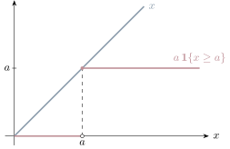
Compare $X$ with the random variable $a\,\mathbf{1}\{X \ge a\}$ pointwise:

if $X \ge a$ : $\;a\,\mathbf{1}\{X \ge a\} = a \le X$ ;
if $X < a$ : $\;a\,\mathbf{1}\{X \ge a\} = 0 \le X$ , since $X \ge 0$ .

So $X \ge a\,\mathbf{1}\{X \ge a\}$ always. Taking expectations, and using $\EE[\mathbf{1}_A] = \PP(A)$ ,

\EE[X] \ge a\,\EE\bigl[\mathbf{1}\{X \ge a\}\bigr] = a\,\PP(X \ge a).

Dividing by $a > 0$ gives (9.1).

The line x lies above the step function a·1{x ≥ a}, which jumps from 0 to a at x = a

For $x \ge 0$ , the line $x$ lies above the step $a\,\mathbf{1}\{x \ge a\}$ ; averaging both sides gives Markov.

Example 9.1 (Markov for an exponential)

Let $X \sim \operatorname{Exponential}(1)$ , so $\EE[X] = 1$ (Lecture 8) and $\PP(X \ge a) = \int_a^\infty e^{-x}\,dx = \Bigl[-e^{-x}\Bigr]_a^\infty = e^{-a}$ . Markov gives

\PP(X \ge a) \le \frac{1}{a}.

At $a = 5$ : Markov gives $0.2$ , while the exact value is $e^{-5} \approx 0.0067$ .

Markov cannot be improved using only the mean. Fix $m = \EE[X]$ and $a \ge m$ . The random variable

X = \begin{cases} a & \text{w.p. } \frac{m}{a}, \\[2pt] 0 & \text{w.p. } 1 - \frac{m}{a} \end{cases}

has $\EE[X] = a \cdot \frac{m}{a} = m$ and $\PP(X \ge a) = \frac{m}{a} = \frac{\EE[X]}{a}$ , so (9.1) holds with equality. To do better, we need more information about $X$ .

Chebyshev’s Inequality

Theorem 9.2 (Chebyshev’s inequality)

If $X$ has mean $\mu$ and variance $\sigma^2$ , then for every $c > 0$ ,

\PP\bigl(|X - \mu| \ge c\bigr) \le \frac{\sigma^2}{c^2}.

With $c = k\sigma$ :

\PP\bigl(|X - \mu| \ge k\sigma\bigr) \le \frac{1}{k^2}.

Proof.

Both sides of $|X - \mu| \ge c$ are nonnegative, so squaring does not change the event: $\{|X - \mu| \ge c\} = \{(X - \mu)^2 \ge c^2\}$ . Apply Markov to the nonnegative random variable $(X - \mu)^2$ with $a = c^2$ :

\PP\bigl(|X - \mu| \ge c\bigr) = \PP\bigl((X - \mu)^2 \ge c^2\bigr) \le \frac{\EE\bigl[(X - \mu)^2\bigr]}{c^2} = \frac{\sigma^2}{c^2}.

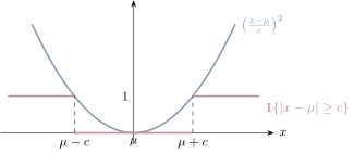
The parabola ((x − μ)/c)² lies above the indicator 1{|x − μ| ≥ c}, which is 1 outside μ ± c and 0 inside

The parabola $\bigl(\frac{x-\mu}{c}\bigr)^2$ lies above the indicator; averaging both sides gives Chebyshev. It uses the variance, not just the mean.

Example 9.2 (Chebyshev for a uniform)

Let $X \sim \operatorname{Uniform}[0,1]$ . Then $\mu = \frac12$ , $\EE[X^2] = \int_0^1 x^2\,dx = \frac13$ , and

\sigma^2 = \EE[X^2] - \mu^2 = \frac13 - \frac14 = \frac{1}{12}.

With $c = 0.4$ , the exact value is $\PP(|X - \tfrac12| \ge 0.4) = \PP(X \le 0.1) + \PP(X \ge 0.9) = 0.1 + 0.1 = 0.2$ , while

\PP\bigl(|X - \tfrac12| \ge 0.4\bigr) \le \frac{1/12}{(0.4)^2} = \frac{1}{12 \cdot 0.16} = \frac{1}{1.92} \approx 0.52.

Example 9.3 (Polling with Chebyshev)

To estimate the fraction $p$ of voters who support a candidate, poll $n$ people independently. Let $X_i \sim \Bern(p)$ indicate support and $M_n = \frac1n\sum_{i=1}^n X_i$ . How large must $n$ be so that $\PP(|M_n - p| \ge 0.01) \le 0.05$ ?

$\EE[M_n] = p$ and $\Var(M_n) = \frac{p(1-p)}{n}$ (Lecture 4 and Lecture 10). Since $p$ is unknown, bound the variance:

p(1 - p) = \frac14 - \Bigl(p - \frac12\Bigr)^2 \le \frac14.

By Chebyshev with $c = \varepsilon$ ,

\PP\bigl(|M_n - p| \ge \varepsilon\bigr) \le \frac{p(1-p)}{n\varepsilon^2} \le \frac{1}{4n\varepsilon^2}.

Setting $\frac{1}{4n\varepsilon^2} \le \delta$ with $\varepsilon = 0.01$ , $\delta = 0.05$ :

n \ge \frac{1}{4\varepsilon^2\delta} = \frac{1}{4\,(0.01)^2\,(0.05)} = \frac{1}{0.00002} = 50{,}000.

The Chernoff Bound

Theorem 9.3 (Chernoff bound)

For every $b$ and every $s > 0$ ,

\PP(X \ge b) \le e^{-sb}\, M_X(s), \qquad M_X(s) = \EE\bigl[e^{sX}\bigr],

and therefore

\PP(X \ge b) \le \min_{s > 0}\; e^{-sb}\, M_X(s).

For the lower tail, $\PP(X \le b) \le \min_{s < 0}\; e^{-sb}\, M_X(s)$ .

Proof.

For $s > 0$ , $x \mapsto e^{sx}$ is strictly increasing, so $\{X \ge b\} = \{e^{sX} \ge e^{sb}\}$ . Apply Markov to the nonnegative random variable $e^{sX}$ :

\PP(X \ge b) = \PP\bigl(e^{sX} \ge e^{sb}\bigr) \le \frac{\EE\bigl[e^{sX}\bigr]}{e^{sb}} = e^{-sb}\, M_X(s).

This holds for every $s > 0$ , so it holds for the minimizing $s$ . For $s < 0$ , $x \mapsto e^{sx}$ is strictly decreasing, so $\{X \le b\} = \{e^{sX} \ge e^{sb}\}$ , and the same argument gives the lower-tail bound.

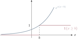
The exponential e^{s(x − b)} lies above the indicator 1{x ≥ b}, which jumps from 0 to 1 at x = b

For any $s > 0$ , the exponential $e^{s(x-b)}$ lies above the indicator $\mathbf{1}\{x \ge b\}$ ; averaging gives $\PP(X \ge b) \le e^{-sb}M_X(s)$ , and we choose $s$ to make the curve hug the indicator as tightly as possible.

Example 9.4 (Gaussian tail)

Let $Z \sim \mathcal{N}(0,1)$ , so $M_Z(s) = e^{s^2/2}$ (Lecture 8). For $t > 0$ ,

\PP(Z \ge t) \le \min_{s > 0}\; e^{-st + s^2/2}.

The exponent $h(s) = \frac{s^2}{2} - st$ has $h'(s) = s - t = 0$ at $s^\star = t$ , and $h(t) = \frac{t^2}{2} - t^2 = -\frac{t^2}{2}$ . Therefore

\PP(Z \ge t) \le e^{-t^2/2}.

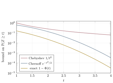
Compare with Chebyshev, which gives $\PP(Z \ge t) \le \PP(|Z| \ge t) \le \frac{1}{t^2}$ :

Log-scale plot for t from 1 to 4 of three curves: Chebyshev 1/t², Chernoff e^{−t²/2}, and the exact tail 1 − Φ(t)

Chebyshev decays polynomially; Chernoff decays like the true tail, up to a smaller factor.

Example 9.5 (Chernoff for coin flips)

Let $S_n \sim \Bin(n, p)$ , a sum of $n$ independent $\Bern(p)$ flips, so $M_{S_n}(s) = \bigl(1 - p + pe^s\bigr)^n$ : each flip has $\EE[e^{sX_i}] = (1-p)e^{0} + pe^{s}$ , and the MGF of an independent sum is the product (Lecture 8). For $p < q < 1$ ,

\PP(S_n \ge qn) \le \min_{s > 0}\; e^{-sqn}\bigl(1 - p + pe^s\bigr)^n = \min_{s > 0}\; \exp\Bigl(n\bigl[-sq + \ln(1 - p + pe^s)\bigr]\Bigr).

Set the derivative of the bracket to zero:

-q + \frac{pe^s}{1 - p + pe^s} = 0 \;\Longrightarrow\; pe^s = q(1 - p + pe^s) \;\Longrightarrow\; pe^s(1 - q) = q(1 - p) \;\Longrightarrow\; e^{s^\star} = \frac{q(1-p)}{p(1-q)},

and $s^\star > 0$ since $q > p$ . At $s^\star$ , $1 - p + pe^{s^\star} = 1 - p + \frac{q(1-p)}{1-q} = \frac{(1-p)(1 - q + q)}{1 - q} = \frac{1-p}{1-q}$ , so the bracket equals

\begin{aligned} -q\ln\frac{q(1-p)}{p(1-q)} + \ln\frac{1-p}{1-q} &= -q\ln\frac{q}{p} - q\ln\frac{1-p}{1-q} + \ln\frac{1-p}{1-q} \\ &= -q\ln\frac{q}{p} + (1 - q)\ln\frac{1-p}{1-q} \\ &= -\Bigl[q\ln\frac{q}{p} + (1 - q)\ln\frac{1-q}{1-p}\Bigr] \triangleq -D(q \,\|\, p). \end{aligned}

Therefore

\PP(S_n \ge qn) \le e^{-n\,D(q \| p)}.

Numbers. $n = 100$ fair flips ( $p = \frac12$ ), at least $75$ heads ( $q = \frac34$ ):

D\bigl(\tfrac34 \,\|\, \tfrac12\bigr) = \tfrac34\ln\tfrac{3/4}{1/2} + \tfrac14\ln\tfrac{1/4}{1/2} = \tfrac34\ln 1.5 + \tfrac14\ln 0.5 \approx 0.304 - 0.173 = 0.131.


Markov	$\frac{\EE[S_n]}{75} = \frac{50}{75}$	$\approx 0.67$
Chebyshev	$\PP(\lvert S_n - 50\rvert \ge 25) \le \frac{\Var(S_n)}{25^2} = \frac{25}{625}$	$= 0.04$
Chernoff	$e^{-100\,D(3/4 \Vert 1/2)} \approx e^{-13.1}$	$\approx 2.1 \times 10^{-6}$
Exact	$\sum_{k=75}^{100}\binom{100}{k}2^{-100}$	$\approx 2.8 \times 10^{-7}$

Jensen’s Inequality

Definition 9.1 (Convex function)

A function $g$ is convex if for all $x, y$ and $\lambda \in [0,1]$ ,

g\bigl(\lambda x + (1 - \lambda)y\bigr) \le \lambda g(x) + (1 - \lambda) g(y): \tag{9.23}

every chord lies above the graph. If $g$ is differentiable, convexity is equivalent to every tangent line lying below the graph:

g(x) \ge g(c) + g'(c)(x - c) \qquad \text{for all } x, c. \tag{9.24}

$g$ is concave if $-g$ is convex. Examples: $x^2$ , $e^{sx}$ , $|x|$ are convex; $\ln x$ and $\sqrt{x}$ are concave on $(0, \infty)$ .

Theorem 9.4 (Jensen’s inequality)

If $g$ is convex, then

g\bigl(\EE[X]\bigr) \le \EE\bigl[g(X)\bigr].

If $g$ is concave, the inequality reverses: $g\bigl(\EE[X]\bigr) \ge \EE\bigl[g(X)\bigr]$ .

Proof.

Take the tangent line (9.24) at $c = \EE[X]$ and substitute $x = X$ :

g(X) \ge g\bigl(\EE[X]\bigr) + g'\bigl(\EE[X]\bigr)\bigl(X - \EE[X]\bigr).

Take expectations. $g(\EE[X])$ and $g'(\EE[X])$ are constants, and $\EE\bigl[X - \EE[X]\bigr] = 0$ :

\EE\bigl[g(X)\bigr] \ge g\bigl(\EE[X]\bigr) + g'\bigl(\EE[X]\bigr) \cdot 0 = g\bigl(\EE[X]\bigr).

(For a convex $g$ that is not differentiable, the same argument works with any supporting line through $(\EE[X], g(\EE[X]))$ .) For concave $g$ , apply the result to $-g$ .

A convex curve g(x) with a chord between x_1 and x_2; at E[X] the chord's midpoint E[g(X)] lies above the curve's value g(E[X]), and the tangent at E[X] lies below the curve

For $X$ equal to $x_1$ or $x_2$ with probability $\frac12$ each, $\EE[g(X)]$ is the midpoint of the chord, which lies above $g(\EE[X])$ on the curve.

Example 9.6 (Consequences of Jensen)

$g(x) = x^2$ (convex): $\bigl(\EE[X]\bigr)^2 \le \EE[X^2]$ , i.e. $\Var(X) = \EE[X^2] - (\EE[X])^2 \ge 0$ .
$g(x) = e^{sx}$ (convex): $e^{s\EE[X]} \le M_X(s)$ , so an MGF is never smaller than $e^{s\EE[X]}$ .
$g(x) = \ln x$ (concave): $\EE[\ln X] \le \ln \EE[X]$ . For $X$ uniform on positive numbers $\{x_1, \ldots, x_n\}$ , $\frac1n \sum_{i=1}^n \ln x_i \le \ln\Bigl(\frac1n\sum_{i=1}^n x_i\Bigr) \;\Longrightarrow\; \Bigl(\prod_{i=1}^n x_i\Bigr)^{1/n} \le \frac1n \sum_{i=1}^n x_i,$ the arithmetic–geometric mean inequality.
In the St. Petersburg game (Lecture 5), $\EE[\log_2 W] = 2$ is finite even though $\EE[W] = \infty$ , consistent with $\EE[\log_2 W] \le \log_2 \EE[W]$ .

Hoeffding’s Inequality

Chernoff requires the MGF. For bounded random variables, we can bound the MGF without knowing the distribution.

Lemma 9.1 (Hoeffding’s lemma)

If $a \le X \le b$ and $\EE[X] = 0$ , then for every $s \in \RR$ ,

\EE\bigl[e^{sX}\bigr] \le e^{s^2 (b - a)^2 / 8}.

Proof.

Since $\EE[X] = 0$ , we have $a \le 0 \le b$ . Write $x \in [a, b]$ as the convex combination $x = \lambda a + (1 - \lambda) b$ with $\lambda = \frac{b - x}{b - a}$ . By convexity of $e^{sx}$ (9.23),

e^{sx} \le \frac{b - x}{b - a}\, e^{sa} + \frac{x - a}{b - a}\, e^{sb}.

Substitute $x = X$ and take expectations, using $\EE[X] = 0$ :

\EE\bigl[e^{sX}\bigr] \le \frac{b}{b - a}\, e^{sa} - \frac{a}{b - a}\, e^{sb}.

Let $p = \frac{-a}{b - a} \in [0, 1]$ and $h = s(b - a)$ , so $sa = -ph$ and $sb = h - ph$ . The right side becomes

(1 - p)\, e^{-ph} + p\, e^{h - ph} = e^{-ph}\bigl(1 - p + pe^h\bigr) = e^{L(h)}, \qquad L(h) = -ph + \ln\bigl(1 - p + pe^h\bigr).

Differentiate:

\begin{aligned} L'(h) &= -p + \frac{pe^h}{1 - p + pe^h}, \qquad L(0) = 0, \qquad L'(0) = -p + p = 0, \\ L''(h) &= \frac{pe^h(1 - p + pe^h) - pe^h \cdot pe^h}{(1 - p + pe^h)^2} = \frac{pe^h}{1 - p + pe^h}\cdot\frac{1 - p}{1 - p + pe^h} = u(1 - u) \le \frac14, \end{aligned}

where $u = \frac{pe^h}{1 - p + pe^h} \in [0,1]$ and $u(1-u) \le \frac14$ (as for $p(1-p)$ above). By Taylor’s theorem with remainder, for some $\xi$ between $0$ and $h$ ,

L(h) = L(0) + L'(0)\,h + \frac{L''(\xi)}{2}\, h^2 \le 0 + 0 + \frac{1}{8}\, h^2 = \frac{s^2(b - a)^2}{8}.

Theorem 9.5 (Hoeffding’s inequality)

Let $X_1, \ldots, X_n$ be independent with $a_i \le X_i \le b_i$ , and $S_n = \sum_{i=1}^n X_i$ . For every $t > 0$ ,

\PP\bigl(S_n - \EE[S_n] \ge t\bigr) \le \exp\Bigl(-\frac{2t^2}{\sum_{i=1}^n (b_i - a_i)^2}\Bigr).

In particular, if the $X_i$ are i.i.d. in $[a, b]$ with mean $\mu$ and $M_n = \frac{S_n}{n}$ ,

\PP\bigl(M_n - \mu \ge \varepsilon\bigr) \le e^{-2n\varepsilon^2/(b-a)^2}, \qquad \PP\bigl(|M_n - \mu| \ge \varepsilon\bigr) \le 2e^{-2n\varepsilon^2/(b-a)^2}. \tag{9.36}

Proof.

Let $C = \sum_i (b_i - a_i)^2$ . Each centered term $X_i - \EE[X_i]$ has mean $0$ and lies in an interval of length $b_i - a_i$ . By Chernoff, independence (Lecture 8), and Hoeffding’s lemma, for $s > 0$ ,

\begin{aligned} \PP\bigl(S_n - \EE[S_n] \ge t\bigr) &\le e^{-st}\, \EE\Bigl[e^{s\sum_i (X_i - \EE[X_i])}\Bigr] = e^{-st} \prod_{i=1}^n \EE\Bigl[e^{s(X_i - \EE[X_i])}\Bigr] \\ &\le e^{-st} \prod_{i=1}^n e^{s^2(b_i - a_i)^2/8} = \exp\Bigl(-st + \frac{s^2 C}{8}\Bigr). \end{aligned}

Minimize the exponent: $-t + \frac{sC}{4} = 0$ at $s^\star = \frac{4t}{C}$ , giving

-\frac{4t}{C}\, t + \frac{16t^2}{C^2}\cdot\frac{C}{8} = -\frac{4t^2}{C} + \frac{2t^2}{C} = -\frac{2t^2}{C}.

For the sample mean, $\{M_n - \mu \ge \varepsilon\} = \{S_n - n\mu \ge n\varepsilon\}$ , so take $t = n\varepsilon$ and $C = n(b-a)^2$ : $\frac{2t^2}{C} = \frac{2n^2\varepsilon^2}{n(b-a)^2} = \frac{2n\varepsilon^2}{(b-a)^2}$ . The lower tail is the same bound applied to $-X_i$ , and adding the two tails gives the factor $2$ .

Example 9.7 (Polling with Hoeffding)

Return to polling: $X_i \in [0, 1]$ , so $b - a = 1$ . By (9.36),

\PP\bigl(|M_n - p| \ge \varepsilon\bigr) \le 2e^{-2n\varepsilon^2} \le \delta \iff n \ge \frac{\ln(2/\delta)}{2\varepsilon^2}.

With $\varepsilon = 0.01$ , $\delta = 0.05$ :

n \ge \frac{\ln 40}{2\,(0.01)^2} = \frac{3.689}{0.0002} \approx 18{,}445,

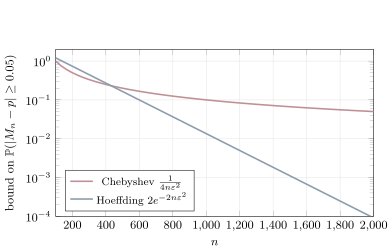
compared with $50{,}000$ from Chebyshev. The two bounds as functions of $n$ (with $\varepsilon = 0.05$ ):

Log-scale plot for n from 100 to 2000: the Chebyshev bound 1/(4nε²) decays like 1/n while the Hoeffding bound 2e^{−2nε²} decays exponentially

Chebyshev decays like $\frac1n$ ; Hoeffding decays exponentially in $n$ .

A First Look at the LLN and the CLT

Law of large numbers. For i.i.d. $X_i$ with mean $\mu$ and variance $\sigma^2$ , Chebyshev gives

\PP\bigl(|M_n - \mu| \ge \varepsilon\bigr) \le \frac{\sigma^2}{n\varepsilon^2} \longrightarrow 0,

which is the weak law of large numbers (proved in full in Lecture 10).

Central limit theorem. $Z_n = \frac{\sqrt{n}\,(M_n - \mu)}{\sigma}$ is approximately $\mathcal{N}(0,1)$ for large $n$ (Lecture 10), so

\PP\bigl(|M_n - \mu| \ge \varepsilon\bigr) = \PP\Bigl(|Z_n| \ge \frac{\varepsilon\sqrt{n}}{\sigma}\Bigr) \approx 2\Bigl(1 - \Phi\Bigl(\frac{\varepsilon\sqrt{n}}{\sigma}\Bigr)\Bigr).

For polling, $\sigma^2 \le \frac14$ , and $2(1 - \Phi(1.96)) = 0.05$ , so we need $\frac{\varepsilon\sqrt{n}}{\sigma} \ge 1.96$ :

n \ge \frac{(1.96)^2\sigma^2}{\varepsilon^2}, \qquad\text{which holds for every } p \text{ once}\qquad n \ge \frac{(1.96)^2}{4\,(0.01)^2} = 9{,}604.

This is an approximation, not a guaranteed bound like Chebyshev or Hoeffding.

Method	Requires	Decay	Polling $n$
Markov	$X \ge 0$ , $\EE[X]$	$1/a$	—
Chebyshev	$\Var(X)$	$1/c^2$ , $1/n$	$50{,}000$
Chernoff	$M_X(s)$	exponential	—
Hoeffding	independent, bounded $X_i$	exponential in $n$	$18{,}445$
CLT	finite variance, large $n$	Gaussian (approximate)	$9{,}604$

concentration-inequalities.html

Lecture 9: Concentration Inequalities

Markov’s Inequality

Chebyshev’s Inequality

The Chernoff Bound

Jensen’s Inequality

Hoeffding’s Inequality

A First Look at the LLN and the CLT