sums-of-random-variables-and-moment-generating-functions.html

Lecture 8: Sums of Independent Random Variables and Moment Generating Functions

EECS 126 (UC Berkeley) · Spring 2026 · February 12, 2026

Reading: Bertsekas & Tsitsiklis, §4.4–4.6.

These are my personal notes from Professor Kannan Ramchandran’s EECS 126 (Probability and Random Processes) course at UC Berkeley.

Topics: sums of independent random variables (convolution), tail bounds, and moment generating functions (MGFs).

Discrete Convolution

Example 8.1 (Sum of two independent discrete random variables)

Let XX and YY be independent, each taking values in {0,1,2,3}\{0, 1, 2, 3\}, with

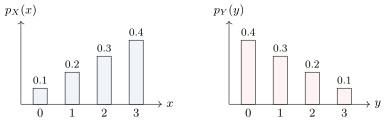
pX=(0.1, 0.2, 0.3, 0.4),pY=(0.4, 0.3, 0.2, 0.1)p_X = (0.1,\ 0.2,\ 0.3,\ 0.4), \qquad p_Y = (0.4,\ 0.3,\ 0.2,\ 0.1)

at the values 0,1,2,30, 1, 2, 3 respectively. Let Z=X+YZ = X + Y. Find P(Z=3)\PP(Z = 3).

Bar charts of the PMFs: p_X = 0.1, 0.2, 0.3, 0.4 and p_Y = 0.4, 0.3, 0.2, 0.1 at the values 0, 1, 2, 3

Z=3Z = 3 occurs exactly for the pairs (x,y)∈{(0,3),(1,2),(2,1),(3,0)}(x, y) \in \{(0,3), (1,2), (2,1), (3,0)\}, i.e. y=3−xy = 3 - x:

P(Z=3)=P(X+Y=3)=∑(x,y) : x+y=3P(X=x, Y=y)=∑(x,y) : x+y=3P(X=x) P(Y=y)(independence)=∑xP(X=x) P(Y=3−x)=pX(0) pY(3)+pX(1) pY(2)+pX(2) pY(1)+pX(3) pY(0)=(0.1)(0.1)+(0.2)(0.2)+(0.3)(0.3)+(0.4)(0.4)=0.01+0.04+0.09+0.16=0.30.\begin{aligned} \PP(Z = 3) = \PP(X + Y = 3) &= \sum_{(x,y)\,:\, x + y = 3} \PP(X = x,\, Y = y) \\ &= \sum_{(x,y)\,:\, x + y = 3} \PP(X = x)\, \PP(Y = y) \qquad \text{(independence)} \\ &= \sum_{x} \PP(X = x)\, \PP(Y = 3 - x) \\ &= p_X(0)\,p_Y(3) + p_X(1)\,p_Y(2) + p_X(2)\,p_Y(1) + p_X(3)\,p_Y(0) \\ &= (0.1)(0.1) + (0.2)(0.2) + (0.3)(0.3) + (0.4)(0.4) \\ &= 0.01 + 0.04 + 0.09 + 0.16 = 0.30. \end{aligned}

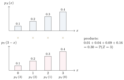
To see the products line up, flip pYp_Y and shift it by 33: plot pY(3−x)p_Y(3 - x) against xx, directly under pX(x)p_X(x), then multiply bar by bar and add.

p_X(x) above the flipped and shifted p_Y(3 − x); multiplying bar by bar gives 0.01 + 0.04 + 0.09 + 0.16 = 0.30 = P(Z = 3)
Definition 8.1 (Discrete convolution)

If XX and YY are independent and integer-valued, then Z=X+YZ = X + Y has PMF

pZ(z)=(pX∗pY)(z)≜∑xpX(x) pY(z−x).(8.3)p_Z(z) = (p_X * p_Y)(z) \triangleq \sum_{x} p_X(x)\, p_Y(z - x). \tag{8.3}

Here xx is a dummy summation variable.

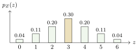
Applying (8.3) at every zz in the example gives the full PMF of ZZ:

Bar chart of the PMF of Z = X + Y: 0.04, 0.11, 0.20, 0.30, 0.20, 0.11, 0.04 at z = 0 through 6, with z = 3 highlighted

Check: 0.04+0.11+0.20+0.30+0.20+0.11+0.04=10.04 + 0.11 + 0.20 + 0.30 + 0.20 + 0.11 + 0.04 = 1.

Continuous Convolution

Theorem 8.1 (Density of a sum of independent random variables)

If XX and YY are independent continuous random variables and Z=X+YZ = X + Y, then

fZ(z)=(fX∗fY)(z)≜∫−∞∞fX(x) fY(z−x) dx.(8.4)f_Z(z) = (f_X * f_Y)(z) \triangleq \int_{-\infty}^{\infty} f_X(x)\, f_Y(z - x)\, dx. \tag{8.4}

Here xx is a dummy variable of integration.

Proof by conditioning.

Find the conditional CDF of ZZ given X=xX = x, then differentiate:

FZ∣X(z∣x)=P(Z≤z∣X=x)=P(X+Y≤z∣X=x)=P(x+Y≤z∣X=x)=P(Y≤z−x∣X=x)=P(Y≤z−x)(independence)=FY(z−x).\begin{aligned} F_{Z \mid X}(z \mid x) = \PP(Z \le z \mid X = x) &= \PP(X + Y \le z \mid X = x) \\ &= \PP(x + Y \le z \mid X = x) \\ &= \PP(Y \le z - x \mid X = x) \\ &= \PP(Y \le z - x) && \text{(independence)} \\ &= F_Y(z - x). \end{aligned}

Differentiating in zz,

fZ∣X(z∣x)=ddzFY(z−x)=fY(z−x).f_{Z \mid X}(z \mid x) = \frac{d}{dz} F_Y(z - x) = f_Y(z - x).

Multiply both sides by the marginal fX(x)f_X(x); the left side becomes the joint PDF of XX and ZZ:

fX,Z(x,z)=fZ∣X(z∣x) fX(x)=fY(z−x) fX(x).f_{X,Z}(x, z) = f_{Z \mid X}(z \mid x)\, f_X(x) = f_Y(z - x)\, f_X(x).

To get the marginal fZf_Z, integrate over all possible xx:

fZ(z)=∫−∞∞fX,Z(x,z) dx=∫−∞∞fX(x) fY(z−x) dx.f_Z(z) = \int_{-\infty}^{\infty} f_{X,Z}(x, z)\, dx = \int_{-\infty}^{\infty} f_X(x)\, f_Y(z - x)\, dx.

Why does the conditioning drop? I was unsure why we can remove “∣X=x\mid X = x”. Once X=xX = x is fixed, the only random variable left in {Y≤z−x}\{Y \le z - x\} is YY, and YY is independent of XX, so conditioning on X=xX = x does not change its distribution.

Proof by a thin strip.

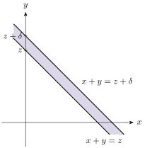
P(z≤Z≤z+δ)\PP(z \le Z \le z + \delta) is the probability that (X,Y)(X, Y) lands in the strip between the lines y=z−xy = z - x and y=z+δ−xy = z + \delta - x:

P(z≤Z≤z+δ)=∫−∞∞∫z−xz−x+δfX,Y(x,y) dy dx=∫−∞∞∫z−xz−x+δfX(x) fY(y) dy dx(independence)=∫−∞∞fX(x)[∫z−xz−x+δfY(y) dy]dx≈∫−∞∞fX(x) fY(z−x) δ dx,\begin{aligned} \PP(z \le Z \le z + \delta) &= \int_{-\infty}^{\infty} \int_{z - x}^{z - x + \delta} f_{X,Y}(x, y)\, dy\, dx \\ &= \int_{-\infty}^{\infty} \int_{z - x}^{z - x + \delta} f_X(x)\, f_Y(y)\, dy\, dx && \text{(independence)} \\ &= \int_{-\infty}^{\infty} f_X(x) \left[\int_{z - x}^{z - x + \delta} f_Y(y)\, dy\right] dx \\ &\approx \int_{-\infty}^{\infty} f_X(x)\, f_Y(z - x)\, \delta\, dx, \end{aligned}

where the inner integral over an interval of width δ\delta is approximated by a rectangle of height fY(z−x)f_Y(z - x). Since also P(z≤Z≤z+δ)≈fZ(z) δ\PP(z \le Z \le z + \delta) \approx f_Z(z)\,\delta,

fZ(z) δ≈∫−∞∞fX(x) fY(z−x) δ dx,f_Z(z)\, \delta \approx \int_{-\infty}^{\infty} f_X(x)\, f_Y(z - x)\, \delta\, dx,

and dividing by δ\delta and letting δ→0\delta \to 0 gives (8.4).

The thin strip between the lines x + y = z and x + y = z + δ in the (x, y) plane

The strip has negative slope because Z=X+YZ = X + Y means Y=Z−XY = Z - X. What we integrate over the strip is the joint density, so P(z≤Z≤z+δ)\PP(z \le Z \le z+\delta) is the probability mass of the strip, not its area.

Example: Sum of Two Uniforms

Example 8.2 (Sum of two independent uniforms)

Let X,Y∼Uniform⁡[0,1]X, Y \sim \operatorname{Uniform}[0,1] be independent, so fX(x)=1b−a=11−0=1f_X(x) = \frac{1}{b - a} = \frac{1}{1 - 0} = 1 on [0,1][0,1], and the same for fYf_Y. Find fZf_Z for Z=X+YZ = X + Y.

By (8.4), writing each density as an indicator,

fZ(z)=∫−∞∞fX(x) fY(z−x) dx=∫−∞∞1{0≤x≤1}⋅1{0≤z−x≤1} dx.f_Z(z) = \int_{-\infty}^{\infty} f_X(x)\, f_Y(z - x)\, dx = \int_{-\infty}^{\infty} \mathbf{1}\{0 \le x \le 1\} \cdot \mathbf{1}\{0 \le z - x \le 1\}\, dx.

The second indicator is 11 when z−1≤x≤zz - 1 \le x \le z. So the integrand is 11 exactly on [max⁡(0,z−1), min⁡(1,z)]\bigl[\max(0, z - 1),\, \min(1, z)\bigr], and fZ(z)f_Z(z) is the length of that interval:

0≤z≤1:fZ(z)=∫0z1 dx=z,1≤z≤2:fZ(z)=∫z−111 dx=1−(z−1)=2−z,\begin{aligned} 0 \le z \le 1: &\quad f_Z(z) = \int_0^{z} 1\, dx = z, \\ 1 \le z \le 2: &\quad f_Z(z) = \int_{z-1}^{1} 1\, dx = 1 - (z - 1) = 2 - z, \end{aligned}

and fZ(z)=0f_Z(z) = 0 otherwise. Check: the triangle has area 12⋅2⋅1=1\tfrac12 \cdot 2 \cdot 1 = 1.

Left: the box f_X(x) on [0, 1] overlapping the sliding box f_Y(z − x) on [z − 1, z]. Right: the triangular density f_Z(z) on [0, 2] with peak 1 at z = 1

Sliding overlap. As a function of xx, fY(z−x)f_Y(z - x) is a box on [z−1,z][z - 1, z] that slides to the right as zz increases. fZ(z)f_Z(z) is the length of its overlap with the box [0,1][0,1]: it grows from 00 at z=0z = 0, is largest at z=1z = 1 (exact overlap), and shrinks back to 00 at z=2z = 2. The same flip-and-slide picture is how convolution is used in signal processing.

Bounding Tail Probabilities

Example 8.3 (How big must a buffer be?)

Over nn time slots, PiP_i packets arrive in slot ii, where P1,…,Pn∼Poisson⁡(1)P_1, \ldots, P_n \sim \Pois(1) are i.i.d. A buffer holds 5n5n packets. How likely is it to overflow? We want to bound

P(∑i=1nPi>5n).\PP\Bigl(\sum_{i=1}^{n} P_i > 5n\Bigr).
Theorem 8.2 (Markov’s inequality)

If X≥0X \ge 0 and a>0a > 0, then

P(X≥a)≤E[X]a.\PP(X \ge a) \le \frac{\EE[X]}{a}.
Proof.

Pointwise, X≥a 1{X≥a}X \ge a\,\mathbf{1}\{X \ge a\}: if X≥aX \ge a the right side is a≤Xa \le X, and otherwise it is 0≤X0 \le X. Taking expectations, E[X]≥a E[1{X≥a}]=a P(X≥a)\EE[X] \ge a\,\EE\bigl[\mathbf{1}\{X \ge a\}\bigr] = a\,\PP(X \ge a).

Let Sn=∑i=1nPi≥0S_n = \sum_{i=1}^n P_i \ge 0. By linearity of expectation and E[Pi]=1\EE[P_i] = 1 for Poisson⁡(1)\Pois(1),

P(Sn>5n)≤P(Sn≥5n)≤E[Sn]5n=∑i=1nE[Pi]5n=∑i=1n15n=n5n=15.\PP(S_n > 5n) \le \PP(S_n \ge 5n) \le \frac{\EE[S_n]}{5n} = \frac{\sum_{i=1}^n \EE[P_i]}{5n} = \frac{\sum_{i=1}^n 1}{5n} = \frac{n}{5n} = \frac15.

Too loose. The bound 15\frac15 does not shrink as nn grows, even though Sn/nS_n/n stays close to its mean 11, far below 55, for large nn. Markov only uses E[Sn]\EE[S_n].

The exponential trick. For t>0t > 0, the function x↦etxx \mapsto e^{tx} is strictly increasing, so the event is unchanged by applying it to both sides. Apply Markov to the nonnegative random variable etSne^{tS_n}:

P(Sn>5n)=P(etSn>e5nt)≤E[etSn]e5nt.(8.16)\PP(S_n > 5n) = \PP\bigl(e^{tS_n} > e^{5nt}\bigr) \le \frac{\EE\bigl[e^{tS_n}\bigr]}{e^{5nt}}. \tag{8.16}

Why etxe^{tx}? I was confused why this particular function. We want to apply a function TT so that E[T(∑iPi)]\EE\bigl[T(\sum_i P_i)\bigr] splits into a product ∏iE[T(Pi)]\prod_i \EE[T(P_i)] by independence. That requires T(x+y)=T(x) T(y)T(x + y) = T(x)\,T(y), which the exponential satisfies: T(x+y)=et(x+y)=etx ety=T(x) T(y)T(x + y) = e^{t(x+y)} = e^{tx}\, e^{ty} = T(x)\,T(y). The parameter t>0t > 0 is a scaling factor we are free to choose.

Since the PiP_i are independent and identically distributed,

E[etSn]=E[etP1+tP2+⋯+tPn]=E[etP1] E[etP2]⋯E[etPn]=(E[etP1])n.\EE\bigl[e^{tS_n}\bigr] = \EE\bigl[e^{tP_1 + tP_2 + \cdots + tP_n}\bigr] = \EE\bigl[e^{tP_1}\bigr]\,\EE\bigl[e^{tP_2}\bigr] \cdots \EE\bigl[e^{tP_n}\bigr] = \Bigl(\EE\bigl[e^{tP_1}\bigr]\Bigr)^n.

For P∼Poisson⁡(λ)P \sim \Pois(\lambda), using the Taylor series ex=∑k≥0xkk!e^{x} = \sum_{k \ge 0} \frac{x^k}{k!},

E[etP]=∑k=0∞etk e−λλkk!=e−λ∑k=0∞(etλ)kk!=e−λ eetλ=eλ(et−1).(8.18)\EE\bigl[e^{tP}\bigr] = \sum_{k=0}^{\infty} e^{tk}\, \frac{e^{-\lambda}\lambda^k}{k!} = e^{-\lambda} \sum_{k=0}^{\infty} \frac{(e^{t}\lambda)^k}{k!} = e^{-\lambda}\, e^{e^t \lambda} = e^{\lambda(e^t - 1)}. \tag{8.18}

Substituting into (8.16),

P(Sn>5n)≤(eλ(et−1))ne5nt=eλn(et−1)−5nt=λ=1e n (et−1−5t).\PP(S_n > 5n) \le \frac{\bigl(e^{\lambda(e^t - 1)}\bigr)^n}{e^{5nt}} = e^{\lambda n (e^t - 1) - 5nt} \overset{\lambda = 1}{=} e^{\,n\,(e^t - 1 - 5t)}.

Choosing tt. The bound holds for every t>0t > 0, so minimize the exponent g(t)=et−1−5tg(t) = e^t - 1 - 5t:

g′(t)=et−5=0  ⟹  t⋆=ln⁡5,g′′(t)=et>0,g'(t) = e^t - 5 = 0 \;\Longrightarrow\; t^\star = \ln 5, \qquad g''(t) = e^t > 0,g(t⋆)=eln⁡5−1−5ln⁡5=4−5ln⁡5≈−4.05.g(t^\star) = e^{\ln 5} - 1 - 5\ln 5 = 4 - 5\ln 5 \approx -4.05.

Therefore

P(∑i=1nPi>5n)≤e−(5ln⁡5−4) n≈e−4.05 n.\PP\Bigl(\sum_{i=1}^n P_i > 5n\Bigr) \le e^{-(5\ln 5 - 4)\,n} \approx e^{-4.05\,n}.

For n=10n = 10: Markov gives 0.20.2, while this bound gives e−40.5≈2.7×10⁻¹⁸e^{-40.5} \approx 2.7 \times 10^{-18}.

Is the bound ∝e−n\propto e^{-n}? I was unsure about the rate. Any t>0t > 0 with g(t)<0g(t) < 0 gives exponential decay eng(t)e^{n g(t)}; the best rate is 5ln⁡5−4≈4.055\ln 5 - 4 \approx 4.05, at t⋆=ln⁡5t^\star = \ln 5. This method (Markov applied to etXe^{tX}, then optimizing over tt) is called the Chernoff bound. The quantity E[etP]\EE[e^{tP}] is the MGF of PP, defined next.

Moment Generating Functions

Definition 8.2 (Moment generating function)

The moment generating function of a random variable XX is

MX(s)≜E[esX]={∑xesx pX(x)(discrete),∫−∞∞esx fX(x) dx(continuous),M_X(s) \triangleq \EE\bigl[e^{sX}\bigr] = \begin{cases} \displaystyle \sum_x e^{sx}\, p_X(x) & \text{(discrete)}, \\[10pt] \displaystyle \int_{-\infty}^{\infty} e^{sx}\, f_X(x)\, dx & \text{(continuous)}, \end{cases}

for s∈Rs \in \RR (it may equal ∞\infty for some ss).

MGFs are useful for:

  1. tight tail bounds (Section 8.4);
  2. computing all the moments E[Xn]\EE[X^n] of a distribution;
  3. sums of independent random variables: convolution becomes multiplication.
Theorem 8.3 (MGFs generate moments)

If MX(s)<∞M_X(s) < \infty for all ss in an open interval around 00, then for every n≥1n \ge 1,

MX(n)(0)=E[Xn].M_X^{(n)}(0) = \EE[X^n].
Proof.

Here ss is a constant inside the expectation and XX is the random part, so ddsesX=XesX\frac{d}{ds} e^{sX} = X e^{sX}. Differentiating nn times and moving the derivative inside the expectation (allowed because MXM_X is finite near 00),

dndsnMX(s)=dndsnE[esX]=E[dndsnesX]=E[XnesX].\frac{d^n}{ds^n} M_X(s) = \frac{d^n}{ds^n} \EE\bigl[e^{sX}\bigr] = \EE\left[\frac{d^n}{ds^n} e^{sX}\right] = \EE\bigl[X^n e^{sX}\bigr].

At s=0s = 0, e0⋅X=e0=1e^{0 \cdot X} = e^0 = 1, so MX(n)(0)=E[XnesX]∣s=0=E[Xn]M_X^{(n)}(0) = \EE\bigl[X^n e^{sX}\bigr]\big|_{s=0} = \EE[X^n].

Example 8.4 (MGF of the exponential)

Let X∼Exponential⁡(λ)X \sim \operatorname{Exponential}(\lambda): fX(x)=λe−λxf_X(x) = \lambda e^{-\lambda x} for x∈[0,∞)x \in [0, \infty). Then

MX(s)=∫0∞esx λe−λx dx=λ∫0∞e(s−λ)x dx.M_X(s) = \int_0^{\infty} e^{sx}\, \lambda e^{-\lambda x}\, dx = \lambda \int_0^{\infty} e^{(s - \lambda)x}\, dx.

If s<λs < \lambda, the exponent s−λs - \lambda is negative and

MX(s)=λ[1s−λ e(s−λ)x]0∞=λ(0−1s−λ)=λλ−s.M_X(s) = \lambda \left[\frac{1}{s - \lambda}\, e^{(s - \lambda)x}\right]_0^{\infty} = \lambda \left(0 - \frac{1}{s - \lambda}\right) = \frac{\lambda}{\lambda - s}.

If s≥λs \ge \lambda, the integrand e(s−λ)x≥1e^{(s-\lambda)x} \ge 1 for all x≥0x \ge 0, so the integral diverges:

MX(s)={λλ−ss<λ,∞s≥λ.M_X(s) = \begin{cases} \dfrac{\lambda}{\lambda - s} & s < \lambda, \\[8pt] \infty & s \ge \lambda. \end{cases}

Moments. MX′(s)=λ(λ−s)2M_X'(s) = \frac{\lambda}{(\lambda - s)^2} and MX′′(s)=2λ(λ−s)3M_X''(s) = \frac{2\lambda}{(\lambda - s)^3}, so

E[X]=MX′(0)=1λ,E[X2]=MX′′(0)=2λ2,Var⁡(X)=2λ2−1λ2=1λ2.\EE[X] = M_X'(0) = \frac{1}{\lambda}, \qquad \EE[X^2] = M_X''(0) = \frac{2}{\lambda^2}, \qquad \Var(X) = \frac{2}{\lambda^2} - \frac{1}{\lambda^2} = \frac{1}{\lambda^2}.
Theorem 8.4 (MGFs determine the distribution)

If MX(s)=MY(s)<∞M_X(s) = M_Y(s) < \infty for all ss in some open interval (−ε,ε)(-\varepsilon, \varepsilon) around 00, then XX and YY have the same distribution.

So if we recognize an MGF, we know the distribution. (The proof is beyond the scope of this course.)

Not finished in lecture. We ran out of time after starting the list of MGF properties. The main properties are filled in below.

Theorem 8.5 (Properties of MGFs)
  1. MX(0)=1M_X(0) = 1.
  2. If Y=aX+bY = aX + b, then MY(s)=esb MX(as)M_Y(s) = e^{sb}\, M_X(as).
  3. If XX and YY are independent, then MX+Y(s)=MX(s) MY(s)M_{X+Y}(s) = M_X(s)\, M_Y(s). More generally, for independent X1,…,XnX_1, \ldots, X_n, MX1+⋯+Xn(s)=∏i=1nMXi(s)M_{X_1 + \cdots + X_n}(s) = \prod_{i=1}^n M_{X_i}(s), and (MX1(s))n\bigl(M_{X_1}(s)\bigr)^n if they are also identically distributed.
Proof.
  1. MX(0)=E[e0⋅X]=E[1]=1M_X(0) = \EE\bigl[e^{0 \cdot X}\bigr] = \EE[1] = 1.
  2. MY(s)=E[es(aX+b)]=E[esb e(as)X]=esb E[e(as)X]=esb MX(as)M_Y(s) = \EE\bigl[e^{s(aX + b)}\bigr] = \EE\bigl[e^{sb}\, e^{(as)X}\bigr] = e^{sb}\, \EE\bigl[e^{(as)X}\bigr] = e^{sb}\, M_X(as), since esbe^{sb} is a constant.
  3. MX+Y(s)=E[es(X+Y)]=E[esX esY]=E[esX] E[esY]=MX(s) MY(s)M_{X+Y}(s) = \EE\bigl[e^{s(X+Y)}\bigr] = \EE\bigl[e^{sX}\, e^{sY}\bigr] = \EE\bigl[e^{sX}\bigr]\,\EE\bigl[e^{sY}\bigr] = M_X(s)\, M_Y(s), using independence of esXe^{sX} and esYe^{sY}. The nn-term version follows by induction.

Property 3 is the payoff: the density of X+YX + Y requires a convolution integral, but its MGF is just a product.

MGF Proofs for Sums of Independent Random Variables

Lemma 8.1 (MGF of the Gaussian)

If X∼N(μ,σ2)X \sim \mathcal{N}(\mu, \sigma^2), then for all s∈Rs \in \RR,

MX(s)=eμs+σ2s2/2.M_X(s) = e^{\mu s + \sigma^2 s^2 / 2}.
Proof.

First let Z∼N(0,1)Z \sim \mathcal{N}(0, 1). Complete the square in the exponent, z2−2sz=(z−s)2−s2z^2 - 2sz = (z - s)^2 - s^2:

MZ(s)=∫−∞∞esz 12π e−z2/2 dz=∫−∞∞12π e−(z2−2sz)/2 dz=∫−∞∞12π e−(z−s)2/2+s2/2 dz=es2/2∫−∞∞12π e−(z−s)2/2 dz=es2/2⋅1,\begin{aligned} M_Z(s) = \int_{-\infty}^{\infty} e^{sz}\, \frac{1}{\sqrt{2\pi}}\, e^{-z^2/2}\, dz &= \int_{-\infty}^{\infty} \frac{1}{\sqrt{2\pi}}\, e^{-(z^2 - 2sz)/2}\, dz \\ &= \int_{-\infty}^{\infty} \frac{1}{\sqrt{2\pi}}\, e^{-(z - s)^2/2 + s^2/2}\, dz \\ &= e^{s^2/2} \int_{-\infty}^{\infty} \frac{1}{\sqrt{2\pi}}\, e^{-(z - s)^2/2}\, dz = e^{s^2/2} \cdot 1, \end{aligned}

since the last integrand is the N(s,1)\mathcal{N}(s, 1) density. Now X=σZ+μX = \sigma Z + \mu (Lecture 7), so by Property 2 with a=σa = \sigma, b=μb = \mu,

MX(s)=eμs MZ(σs)=eμs eσ2s2/2=eμs+σ2s2/2.M_X(s) = e^{\mu s}\, M_Z(\sigma s) = e^{\mu s}\, e^{\sigma^2 s^2/2} = e^{\mu s + \sigma^2 s^2/2}.
Theorem 8.6 (Sum of independent Gaussians)

If X∼N(μX,σX2)X \sim \mathcal{N}(\mu_X, \sigma_X^2) and Y∼N(μY,σY2)Y \sim \mathcal{N}(\mu_Y, \sigma_Y^2) are independent, then

X+Y∼N(μX+μY,  σX2+σY2).X + Y \sim \mathcal{N}\bigl(\mu_X + \mu_Y,\; \sigma_X^2 + \sigma_Y^2\bigr).
Proof.

By Property 3 and the Gaussian MGF,

MX+Y(s)=MX(s) MY(s)=eμXs+σX2s2/2⋅eμYs+σY2s2/2=e(μX+μY)s+(σX2+σY2)s2/2,\begin{aligned} M_{X+Y}(s) = M_X(s)\, M_Y(s) &= e^{\mu_X s + \sigma_X^2 s^2/2} \cdot e^{\mu_Y s + \sigma_Y^2 s^2/2} \\ &= e^{(\mu_X + \mu_Y)s + (\sigma_X^2 + \sigma_Y^2)s^2/2}, \end{aligned}

which is the MGF of N(μX+μY, σX2+σY2)\mathcal{N}(\mu_X + \mu_Y,\, \sigma_X^2 + \sigma_Y^2), finite for all ss. Since MGFs determine the distribution, X+Y∼N(μX+μY, σX2+σY2)X + Y \sim \mathcal{N}(\mu_X + \mu_Y,\, \sigma_X^2 + \sigma_Y^2).

This completes the proof left as TBD in Lecture 7.

Corollary 8.1 (Sum of independent Poissons)

If X∼Poisson⁡(λ)X \sim \Pois(\lambda) and Y∼Poisson⁡(μ)Y \sim \Pois(\mu) are independent, then X+Y∼Poisson⁡(λ+μ)X + Y \sim \Pois(\lambda + \mu).

Proof.

By (8.18), MX(s)=eλ(es−1)M_X(s) = e^{\lambda(e^s - 1)} and MY(s)=eμ(es−1)M_Y(s) = e^{\mu(e^s - 1)}, so

MX+Y(s)=eλ(es−1) eμ(es−1)=e(λ+μ)(es−1),M_{X+Y}(s) = e^{\lambda(e^s - 1)}\, e^{\mu(e^s - 1)} = e^{(\lambda + \mu)(e^s - 1)},

the MGF of Poisson⁡(λ+μ)\Pois(\lambda + \mu). (Compare the convolution proof of Poisson merging in Lecture 4.)

2380 words