Lecture 7: The Gaussian Distribution, Derived Distributions, and Order Statistics

EECS 126 (UC Berkeley) · Spring 2026 · February 10, 2026

Reading: Bertsekas & Tsitsiklis, §3.3, §4.1.

These are my personal notes from Professor Kannan Ramchandran’s EECS 126 (Probability and Random Processes) course at UC Berkeley.

Topics: the Gaussian distribution, change of variables (derived distributions), and order statistics.

The Gaussian Distribution

Definition 7.1 (Gaussian (normal) distribution)

$X \sim \mathcal{N}(\mu, \sigma^2)$ , with $\mu \in \RR$ and $\sigma > 0$ , if

f_X(x) = \frac{1}{\sqrt{2\pi}\,\sigma}\, e^{-(x-\mu)^2/2\sigma^2}, \qquad x \in \RR.

The standard normal is $Z \sim \mathcal{N}(0, 1)$ :

f_Z(z) = \frac{1}{\sqrt{2\pi}}\, e^{-z^2/2}, \qquad z \in \RR. \tag{7.2}

The constant $\frac{1}{\sqrt{2\pi}}$ is the normalization factor that makes $\int_{-\infty}^{\infty} f_Z(z)\,dz = 1$ .

Definition 7.2 (Standard normal CDF)

\Phi(z) \triangleq \PP(Z \le z) = \int_{-\infty}^{z} \frac{1}{\sqrt{2\pi}}\, e^{-u^2/2}\, du.

$u$ is a dummy variable of integration; $z$ appears only in the upper limit. $\Phi$ has no closed form, so its values are read from a table.

Theorem 7.1 (Key Gaussian integral)

For every $\alpha > 0$ ,

\int_{-\infty}^{\infty} e^{-\alpha x^2/2}\, dx = \sqrt{\frac{2\pi}{\alpha}},

or equivalently

I(\alpha) \triangleq \frac{1}{\sqrt{2\pi}} \int_{-\infty}^{\infty} e^{-\alpha x^2/2}\, dx = \frac{1}{\sqrt{\alpha}} = \alpha^{-1/2}. \tag{7.5}

Proof.

Substitute $u = \sqrt{\alpha}\,x$ , so $du = \sqrt{\alpha}\,dx$ and $\alpha x^2 = u^2$ :

\int_{-\infty}^{\infty} e^{-\alpha x^2/2}\, dx = \int_{-\infty}^{\infty} e^{-u^2/2}\, \frac{du}{\sqrt{\alpha}} = \frac{1}{\sqrt{\alpha}} \int_{-\infty}^{\infty} e^{-u^2/2}\, du = \frac{1}{\sqrt{\alpha}} \cdot \sqrt{2\pi},

where the last step uses $\int_{-\infty}^{\infty} \frac{1}{\sqrt{2\pi}} e^{-u^2/2}\,du = 1$ from (7.2). Dividing by $\sqrt{2\pi}$ gives (7.5).

Mean and Variance of the Standard Normal

Theorem 7.2 (Standard normal moments)

If $Z \sim \mathcal{N}(0,1)$ , then $\EE[Z] = 0$ and $\Var(Z) = 1$ .

Proof of 𝔼[Z] = 0.

\EE[Z] = \int_{-\infty}^{\infty} z\, f_Z(z)\, dz = \int_{-\infty}^{\infty} \frac{1}{\sqrt{2\pi}}\, z\, e^{-z^2/2}\, dz.

The integrand $g(z) = z\,e^{-z^2/2}$ is odd, $g(-z) = -g(z)$ , so the two halves cancel:

\begin{aligned} \int_{0}^{\infty} z\, e^{-z^2/2}\, dz &= \Bigl[-e^{-z^2/2}\Bigr]_0^{\infty} = 0 - (-1) = 1, \\ \int_{-\infty}^{0} z\, e^{-z^2/2}\, dz &= \Bigl[-e^{-z^2/2}\Bigr]_{-\infty}^{0} = -1 - 0 = -1, \end{aligned}

and therefore $\EE[Z] = \frac{1}{\sqrt{2\pi}}(1 - 1) = 0$ .

Proof of Var(Z) = 1.

Differentiate $e^{-\alpha x^2/2}$ with respect to $\alpha$ :

\frac{d}{d\alpha}\Bigl(e^{-\alpha x^2/2}\Bigr) = -\frac{x^2}{2}\, e^{-\alpha x^2/2} \quad\Longrightarrow\quad x^2 e^{-\alpha x^2/2} = -2\, \frac{d}{d\alpha}\Bigl(e^{-\alpha x^2/2}\Bigr).

Then

\begin{aligned} \EE[Z^2] &= \int_{-\infty}^{\infty} x^2\, \frac{1}{\sqrt{2\pi}}\, e^{-x^2/2}\, dx \\ &= \left[\int_{-\infty}^{\infty} \frac{1}{\sqrt{2\pi}}\, x^2 e^{-\alpha x^2/2}\, dx\right]_{\alpha=1} \\ &= \left[\int_{-\infty}^{\infty} \frac{-2}{\sqrt{2\pi}}\, \frac{d}{d\alpha}\Bigl(e^{-\alpha x^2/2}\Bigr)\, dx\right]_{\alpha=1} \\ &= \left[-2\, \frac{d}{d\alpha}\left(\frac{1}{\sqrt{2\pi}} \int_{-\infty}^{\infty} e^{-\alpha x^2/2}\, dx\right)\right]_{\alpha=1} && \text{(Leibniz rule)} \\ &= \left[-2\, \frac{d}{d\alpha}\, I(\alpha)\right]_{\alpha=1} = \left[-2\, \frac{d}{d\alpha}\, \alpha^{-1/2}\right]_{\alpha=1} && \text{by (7.5)} \\ &= \left[-2 \left(-\tfrac12\, \alpha^{-3/2}\right)\right]_{\alpha=1} = \left[\alpha^{-3/2}\right]_{\alpha=1} = \left[\frac{1}{\sqrt{\alpha^3}}\right]_{\alpha=1} = 1. \end{aligned}

The Leibniz rule (differentiation under the integral sign) justifies moving $\frac{d}{d\alpha}$ outside the integral. Finally,

\Var(Z) = \EE[Z^2] - (\EE[Z])^2 = 1 - 0^2 = 1.

Why only $\alpha = 1$ ? I was confused why we set $\alpha = 1$ , and whether it could be something else. The identity $I(\alpha) = \alpha^{-1/2}$ holds for every $\alpha > 0$ , so $I$ is a function of $\alpha$ that we can differentiate, and differentiating in $\alpha$ is what produces the factor $x^2$ . We set $\alpha = 1$ only after differentiating, because the standard normal has $e^{-x^2/2}$ , i.e. $\alpha = 1$ . Setting $\alpha = 1$ first would leave the constant $I(1) = 1$ , whose derivative is $0$ .

Cross-check by integration by parts. With $u = x$ and $dv = \frac{1}{\sqrt{2\pi}}\, x e^{-x^2/2}\,dx$ , so $v = -\frac{1}{\sqrt{2\pi}}\, e^{-x^2/2}$ :

\EE[Z^2] = \left[-\frac{x}{\sqrt{2\pi}}\, e^{-x^2/2}\right]_{-\infty}^{\infty} + \int_{-\infty}^{\infty} \frac{1}{\sqrt{2\pi}}\, e^{-x^2/2}\, dx = 0 + 1 = 1.

Linear Transformations of Gaussians

Theorem 7.3 (Shifting and scaling a standard normal)

If $Z \sim \mathcal{N}(0,1)$ , $\sigma > 0$ , and $X = \sigma Z + \mu$ , then $X \sim \mathcal{N}(\mu, \sigma^2)$ .

Proof.

Start with the CDF of $X$ . Since $\sigma > 0$ , dividing by $\sigma$ preserves the inequality:

F_X(x) = \PP(X \le x) = \PP(\sigma Z + \mu \le x) = \PP\left(Z \le \frac{x - \mu}{\sigma}\right) = F_Z(z), \qquad z = \frac{x - \mu}{\sigma}.

Differentiate with the chain rule, using $\frac{dz}{dx} = \frac{d}{dx}\left(\frac{x}{\sigma} - \frac{\mu}{\sigma}\right) = \frac{1}{\sigma}$ :

\begin{aligned} f_X(x) = \frac{d}{dx} F_X(x) = \frac{d}{dx} F_Z(z) = f_Z(z)\, \frac{dz}{dx} &= \frac{1}{\sqrt{2\pi}}\, e^{-z^2/2} \cdot \frac{1}{\sigma} \\ &= \frac{1}{\sqrt{2\pi}\,\sigma}\, e^{-(x-\mu)^2/2\sigma^2}. \end{aligned}

Is $f_Z(z) \cdot \frac{1}{\sigma}$ already the answer? I was unsure whether the line $f_X(x) = \frac{1}{\sqrt{2\pi}} e^{-z^2/2} \cdot \frac{1}{\sigma}$ was correct. It is: substituting $z = \frac{x-\mu}{\sigma}$ gives exactly the $\mathcal{N}(\mu, \sigma^2)$ density. The factor $\frac{1}{\sigma}$ in front comes from $\frac{dz}{dx}$ .

Should $\mu$ and $\sigma$ have a subscript $Z$ ? I was also confused about this. No: $Z$ always has mean $0$ and variance $1$ . Here $\mu$ and $\sigma$ are the shift and scale applied to $Z$ , and they become the mean and standard deviation of $X$ : $\EE[X] = \sigma\,\EE[Z] + \mu = \mu$ and $\Var(X) = \sigma^2 \Var(Z) = \sigma^2$ . If anything, they are $\mu_X$ and $\sigma_X$ .

Corollary 7.1 (Standardization)

If $X \sim \mathcal{N}(\mu, \sigma^2)$ , then $Z = \dfrac{X - \mu}{\sigma} \sim \mathcal{N}(0, 1)$ , and

F_X(x) = \Phi\!\left(\frac{x - \mu}{\sigma}\right).

Symmetry of Φ and Standardization

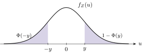
Theorem 7.4 (Symmetry of the standard normal CDF)

For every $y \in \RR$ ,

\Phi(-y) = 1 - \Phi(y).

So a table only needs $\Phi(y)$ for $y \ge 0$ .

Proof.

$f_Z$ is even: $f_Z(-v) = f_Z(v)$ . Substitute $u = -v$ , $du = -dv$ :

\begin{aligned} \Phi(-y) = \int_{-\infty}^{-y} f_Z(u)\, du &= \int_{\infty}^{y} f_Z(-v)\,(-dv) = \int_{y}^{\infty} f_Z(v)\, dv \\ &= \PP(Z \ge y) = 1 - \PP(Z < y) = 1 - \Phi(y), \end{aligned}

using $\PP(Z < y) = \PP(Z \le y)$ for a continuous random variable.

Standard normal density with equal shaded tails: the left tail below −y is Φ(−y) and the right tail above y is 1 − Φ(y)

Example 7.1 (Annual rainfall)

The annual rainfall in a city is $X \sim \mathcal{N}(60, 20^2)$ , in inches. Find $\PP(X > 80)$ .

Standardize with $Z = \frac{X - 60}{20} \sim \mathcal{N}(0,1)$ :

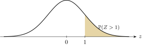
\begin{aligned} \PP(X > 80) &= \PP\left(\frac{X - 60}{20} > \frac{80 - 60}{20}\right) \\ &= \PP\left(\frac{X - 60}{20} > 1\right) = \PP(Z > 1) \\ &= 1 - \PP(Z \le 1) = 1 - \Phi(1) = 1 - 0.8413 = 0.1587. \end{aligned}

Standard normal density with the right tail above z = 1 shaded, labeled P(Z > 1)

Why $1 - \Phi(1)$ ? I was confused why the answer is $1 - \Phi(1)$ rather than $\Phi(1)$ . $\Phi(1)$ is the area to the left of $1$ ; $\PP(Z > 1)$ is the area to the right, which is its complement.

Sums of Independent Gaussians

Theorem 7.5 (Sum of independent Gaussians)

If $X \sim \mathcal{N}(\mu_X, \sigma_X^2)$ and $Y \sim \mathcal{N}(\mu_Y, \sigma_Y^2)$ are independent, then

X + Y \sim \mathcal{N}\bigl(\mu_X + \mu_Y,\; \sigma_X^2 + \sigma_Y^2\bigr).

The parameters follow from Lecture 4: $\EE[X+Y] = \EE[X] + \EE[Y] = \mu_X + \mu_Y$ , and by independence $\Var(X+Y) = \Var(X) + \Var(Y) = \sigma_X^2 + \sigma_Y^2$ . The content of the theorem is that $X + Y$ is again Gaussian. This can be shown with a convolution, or in one line with moment generating functions.

Proof: MGF proof TBD in a later lecture.

Theorem 7.6 (Converse)

If $X$ and $Y$ are independent and $X + Y$ is Gaussian, then $X$ and $Y$ are each Gaussian (allowing a constant, i.e. variance $0$ ).

This direction is much harder; its proof is beyond the scope of this course.

Derived Distributions

Given $X$ with known density $f_X$ and $Y = g(X)$ , find $f_Y$ .

Theorem 7.7 (CDF method)

F_Y(y) = \PP(Y \le y) = \PP\bigl(g(X) \le y\bigr) = \PP\bigl(X \in \{x : g(x) \le y\}\bigr) = \int_{\{x \,:\, g(x) \le y\}} f_X(x)\, dx,

and then

f_Y(y) = \frac{dF_Y(y)}{dy}.

If $g$ is strictly increasing, $\{x : g(x) \le y\} = \{x \le g^{-1}(y)\}$ , so $F_Y(y) = F_X\bigl(g^{-1}(y)\bigr)$ . If $g$ is strictly decreasing, the inequality flips: $\{x : g(x) \le y\} = \{x \ge g^{-1}(y)\}$ , so $F_Y(y) = 1 - F_X\bigl(g^{-1}(y)\bigr)$ .

Corollary 7.2 (Monotone change of variables)

If $g$ is strictly monotone and differentiable, then

f_Y(y) = f_X\bigl(g^{-1}(y)\bigr) \left| \frac{d\, g^{-1}(y)}{dy} \right|. \tag{7.21}

Proof.

Increasing $g$ : $\frac{d}{dy} F_X(g^{-1}(y)) = f_X(g^{-1}(y)) \frac{d g^{-1}(y)}{dy}$ , with $\frac{d g^{-1}(y)}{dy} > 0$ . Decreasing $g$ : $\frac{d}{dy}\bigl[1 - F_X(g^{-1}(y))\bigr] = -f_X(g^{-1}(y)) \frac{d g^{-1}(y)}{dy}$ , with $\frac{d g^{-1}(y)}{dy} < 0$ . In both cases the result is (7.21).

For $X = \sigma Z + \mu$ : $g^{-1}(x) = \frac{x-\mu}{\sigma}$ and $\frac{d g^{-1}(x)}{dx} = \frac{1}{\sigma}$ , which is the factor $\frac{1}{\sigma}$ found in Section 7.3.

Example 7.2 (Square root of a uniform)

Let $X \sim \operatorname{Uniform}[0,1]$ and $Y = \sqrt{X}$ . For $0 \le y \le 1$ , since $\sqrt{x}$ is increasing on $[0,1]$ and both sides are nonnegative,

F_Y(y) = \PP(Y \le y) = \PP(\sqrt{X} \le y) = \PP(X \le y^2) = F_X(y^2) = \int_0^{y^2} 1\, dx = \Bigl[x\Bigr]_0^{y^2} = y^2 - 0 = y^2,

with $F_Y(y) = 0$ for $y < 0$ and $F_Y(y) = 1$ for $y > 1$ . Differentiating,

f_Y(y) = \frac{d}{dy} F_Y(y) = \frac{d}{dy}\bigl(y^2\bigr) = 2y, \qquad 0 \le y \le 1.

Check with (7.21): $g^{-1}(y) = y^2$ , $\frac{d g^{-1}(y)}{dy} = 2y$ , $f_X(y^2) = 1$ , so $f_Y(y) = 1 \cdot 2y = 2y$ .

$Y = \sqrt{X}$ has the same density $2y$ as the distance of a random dart from the center of the unit disk (Lecture 5).

Order Statistics

Let $X_1, X_2, \ldots, X_n$ be i.i.d. samples with common density $f_X$ and CDF $F_X$ .

Definition 7.3 (Order statistics)

X^{(k)} \triangleq \text{the } k\text{-th smallest of } X_1, X_2, \ldots, X_n, \qquad k = 1, \ldots, n.

In particular $X^{(1)} = \min_i X_i$ and $X^{(n)} = \max_i X_i$ .

Example 7.3 (Ordering three samples)

$n = 3$ , $X_i \sim \operatorname{Uniform}(0,1)$ , observed $(X_1, X_2, X_3) = (0.3,\, 0.8,\, 0.4)$ . Then

X^{(1)} = 0.3, \qquad X^{(2)} = 0.4, \qquad X^{(3)} = 0.8.

Question: what is $f_{X^{(k)}}(x)$ , the density of $X^{(k)}$ ?

By the definition of a density,

\PP\bigl(X^{(k)} \in (x, x + dx)\bigr) \approx f_{X^{(k)}}(x)\, dx.

For the $k$ -th smallest sample to lie in $(x, x+dx)$ , we need

$k - 1$ samples in $(-\infty, x)$ : probability $\bigl[F_X(x)\bigr]^{k-1}$ ;
$1$ sample in $(x, x + dx)$ : probability $f_X(x)\,dx$ ;
$n - k$ samples in $(x + dx, \infty)$ : probability $\bigl[1 - F_X(x)\bigr]^{n-k}$ ,

where the probabilities multiply by independence.

Number line with k − 1 samples left of x, the k-th order statistic in the interval (x, x + dx), and n − k samples to the right

Count the ways to assign the $n$ samples to the three regions:

which sample lies in $(x, x+dx)$ : $n$ ways;
which $k-1$ of the remaining $n-1$ lie to the left: $\binom{n-1}{k-1}$ ways;
the remaining $n-k$ lie to the right: $1$ way.

n \binom{n-1}{k-1} = n \cdot \frac{(n-1)!}{(k-1)!\,\bigl((n-1)-(k-1)\bigr)!} = \frac{n!}{(k-1)!\,(n-k)!}.

Why only $1$ way for the third group? I was confused whether the right-hand group contributes $\binom{\,\cdot\,}{n-k}$ more choices. It does not: once the middle sample and the $k-1$ left samples are chosen, the other $n-k$ samples are forced to the right. (Two or more samples landing in $(x, x+dx)$ has probability of order $(dx)^2$ , which is negligible.)

Theorem 7.8 (Density of the

k

-th order statistic)

f_{X^{(k)}}(x) = \frac{n!}{(k-1)!\,(n-k)!}\, \bigl[F_X(x)\bigr]^{k-1} \bigl[1 - F_X(x)\bigr]^{n-k} f_X(x). \tag{7.28}

Proof.

Multiply the number of assignments by the probability of each:

f_{X^{(k)}}(x)\, dx = \frac{n!}{(k-1)!\,(n-k)!}\, \bigl[F_X(x)\bigr]^{k-1} \bigl[1 - F_X(x)\bigr]^{n-k} f_X(x)\, dx,

and divide both sides by $dx$ .

Why $y$ ? I was confused why the formula was written in $y$ rather than $x$ . The argument is a dummy variable: $f_{X^{(k)}}(y)$ and $f_{X^{(k)}}(x)$ are the same function. What matters is that one variable is used throughout, and that $F_X$ and $f_X$ are the CDF and PDF of a single sample, not of $X^{(k)}$ .

Check, $k = n$ (the maximum). $\PP(X^{(n)} \le x) = \PP(\text{all } X_i \le x) = \bigl[F_X(x)\bigr]^n$ , and $\frac{d}{dx}\bigl[F_X(x)\bigr]^n = n\bigl[F_X(x)\bigr]^{n-1} f_X(x)$ , matching (7.28) with $k = n$ .

Corollary 7.3 (Uniform samples)

If $X_i \sim \operatorname{Uniform}[0,1]$ , then $f_X(x) = 1$ and $F_X(x) = x$ on $[0,1]$ , so

f_{X^{(k)}}(x) = \frac{n!}{(k-1)!\,(n-k)!}\, x^{k-1} (1 - x)^{n-k}, \qquad 0 \le x \le 1. \tag{7.30}

On [0, 1], the Uniform density f_X(x) = 1 is a flat line and the CDF F_X(x) = x is the diagonal

Example 7.4 (Third smallest of four uniforms)

$X_i \sim \operatorname{Uniform}[0,1]$ , $n = 4$ . Find $\PP\bigl(X^{(3)} < \tfrac12\bigr)$ .

With $n = 4$ , $k = 3$ : $\frac{n!}{(k-1)!\,(n-k)!} = \frac{4!}{2!\,1!} = \frac{24}{2} = 12$ . By (7.30),

\begin{aligned} \PP\bigl(X^{(3)} < \tfrac12\bigr) = F_{X^{(3)}}\bigl(\tfrac12\bigr) &= \int_0^{1/2} f_{X^{(3)}}(x)\, dx = \int_0^{1/2} 12\, x^2 (1 - x)\, dx \\ &= 12 \int_0^{1/2} \bigl(x^2 - x^3\bigr)\, dx = 12 \left[\frac{x^3}{3} - \frac{x^4}{4}\right]_0^{1/2} \\ &= 12 \left(\frac{1}{24} - \frac{1}{64}\right) = 12 \left(\frac{8}{192} - \frac{3}{192}\right) = 12 \cdot \frac{5}{192} = \frac{60}{192} = \frac{5}{16}. \end{aligned}

Check: $X^{(3)} < \tfrac12$ exactly when at least $3$ of the $4$ samples are below $\tfrac12$ . The number below $\tfrac12$ is $\Bin(4, \tfrac12)$ , so

\PP\bigl(X^{(3)} < \tfrac12\bigr) = \binom{4}{3}\Bigl(\tfrac12\Bigr)^4 + \binom{4}{4}\Bigl(\tfrac12\Bigr)^4 = \frac{4}{16} + \frac{1}{16} = \frac{5}{16}.

Example 7.5 (Expected minimum by symmetry)

$X_i \sim \operatorname{Uniform}[0,1]$ , $n = 10$ . Find $\EE[X^{(1)}]$ , the expected smallest sample.

The $10$ samples cut $[0,1]$ into $11$ gaps:

\Delta_1 = X^{(1)} - 0, \qquad \Delta_i = X^{(i)} - X^{(i-1)} \;\; (2 \le i \le 10), \qquad \Delta_{11} = 1 - X^{(10)}.

Ten points on [0, 1] labeled X^(1) through X^(10), cutting the interval into gaps Δ1 through Δ11

The sum telescopes:

\sum_{i=1}^{11} \Delta_i = (X^{(1)} - 0) + (X^{(2)} - X^{(1)}) + \cdots + (X^{(10)} - X^{(9)}) + (1 - X^{(10)}) = 1.

By symmetry, all $11$ gaps have the same distribution, so $\EE[\Delta_i] = \EE[\Delta_1]$ for every $i$ . Taking expectations,

\EE\Bigl[\sum_{i=1}^{11} \Delta_i\Bigr] = \sum_{i=1}^{11} \EE[\Delta_i] = 11\, \EE[\Delta_1] = \EE[1] = 1 \quad\Longrightarrow\quad \EE[X^{(1)}] = \EE[\Delta_1] = \frac{1}{11}.

Do the gaps really sum to $1$ ? I was unsure about this. They do: the gaps tile $[0,1]$ exactly, which is the telescoping sum above.

Why are the gaps symmetric? Place $11$ independent uniform points on a circle of circumference $1$ and cut the circle at one of them. The other $10$ points are i.i.d. uniform on the resulting interval $[0,1]$ , and the $11$ arcs between consecutive points are exactly the gaps $\Delta_1, \ldots, \Delta_{11}$ . On the circle no arc is special, so all gaps have the same distribution.

Cross-check with (7.30). With $k = 1$ : $f_{X^{(1)}}(x) = \frac{10!}{0!\,9!}(1-x)^9 = 10(1-x)^9$ . Substituting $u = 1 - x$ ,

\EE[X^{(1)}] = \int_0^1 x \cdot 10(1-x)^9\, dx = \int_0^1 (1 - u)\, 10\, u^9\, du = 10\left(\frac{1}{10} - \frac{1}{11}\right) = 10 \cdot \frac{1}{110} = \frac{1}{11}.

General case. $X^{(k)} = \Delta_1 + \cdots + \Delta_k$ , so for $n$ uniform samples,

\EE[X^{(k)}] = k\, \EE[\Delta_1] = \frac{k}{n+1}.

Next lecture: moment generating functions (MGFs).

gaussian-derived-distributions-and-order-statistics.html

Lecture 7: The Gaussian Distribution, Derived Distributions, and Order Statistics

The Gaussian Distribution

Mean and Variance of the Standard Normal

Linear Transformations of Gaussians

Symmetry of Φ and Standardization

Sums of Independent Gaussians

Derived Distributions

Order Statistics