Lecture 5: Iterated Expectation, Conditional Variance, and Continuous Random Variables

EECS 126 (UC Berkeley) · Spring 2026 · February 3, 2026

Reading: Bertsekas & Tsitsiklis, §4.2–4.3; Ch. 3.

These are my personal notes from Professor Kannan Ramchandran’s EECS 126 (Probability and Random Processes) course at UC Berkeley.

We open with a famous game whose expected payout is infinite. We then finish the story of conditional expectation from Lecture 4: the law of iterated expectation (the tower rule), which we use to analyze a random walk, and its companion for variances, the law of total variance. The second half of the lecture moves from discrete to continuous random variables, introducing probability density functions (PDFs) and cumulative distribution functions (CDFs).

The St. Petersburg Paradox

Example 5.1 (St. Petersburg game)

I toss a fair coin until I get a heads. If I toss $n$ times, I give you $\text{\textdollar}2^n$ . For example,

H \;\mapsto\; \$2, \qquad TH \;\mapsto\; \$4, \qquad TTH \;\mapsto\; \$8, \qquad \ldots

Question: how much would you pay to play this game?

Let $N$ be the number of tosses in the game and $W = 2^N$ the amount of money you win. The game ends on the first heads, so $N \sim \Geom(\tfrac12)$ :

\PP(N = n) = \underbrace{\tfrac12 \cdot \tfrac12 \cdots \tfrac12}_{n \text{ flips}} = 2^{-n}, \qquad n = 1, 2, 3, \ldots

(The first $n - 1$ flips are tails and the $n$ -th is heads; each has probability $\tfrac12$ .) By LOTUS,

\EE[W] = \sum_{n=1}^{\infty} 2^n \cdot \PP(N = n) = \sum_{n=1}^{\infty} 2^n \cdot \frac{1}{2^n} = \sum_{n=1}^{\infty} 1 = \infty.

The expected payout is infinite. This is the St. Petersburg paradox.

Why is it a paradox? If expected value were the whole story, you should be willing to pay any finite price to play. Yet almost nobody would pay more than a few dollars: half the time the game pays $\text{\textdollar}2$ , and $\PP(W \le \text{\textdollar}8) = \tfrac78$ . The infinite mean is driven entirely by astronomically rare, astronomically large payouts (each outcome $n$ contributes exactly $\text{\textdollar}1$ to the mean). Two standard resolutions:

Diminishing utility. Daniel Bernoulli argued that the value of money grows more slowly than the amount, e.g. logarithmically. The expected log-payout is finite: $\EE[\log_2 W] = \EE[N] = 2$ (the geometric mean from Lecture 4), which corresponds to a “fair price” of about $2^2 = \text{\textdollar}4$ .
Finite bankroll. No casino can pay more than some $\text{\textdollar}2^M$ . If payouts are capped at $2^M$ , then $\EE[W] = \sum_{n=1}^{M} 2^n 2^{-n} + \sum_{n=M+1}^{\infty} 2^M 2^{-n} = M + 2^M \cdot 2^{-M} = M + 1.$ Even a billion-dollar bankroll ( $2^{30} \approx 1.07\times 10^9$ ) gives an expected payout of only $\text{\textdollar}31$ .

Conditional Expectation as a Random Variable

Recall from Lecture 4 that for each value $y$ with $\PP(Y = y) > 0$ ,

\EE[X \mid Y = y] = \sum_x x \cdot \PP(X = x \mid Y = y)

is a number. Letting $g(y) = \EE[X \mid Y = y]$ , the conditional expectation $\EE[X \mid Y] \triangleq g(Y)$ is a function of $Y$ , and therefore $\EE[X \mid Y]$ is a random variable.

Example 5.2 (Tossing a fair coin a random number of times)

We toss a fair coin $N$ times, where $N$ is itself a random variable taking values in $\{1, 2, 3, \ldots\}$ . Let $X$ be the total number of heads. Given $N = n$ , the $n$ tosses are independent fair Bernoulli trials, so $X \mid N = n \sim \Bin(n, \tfrac12)$ .

$N = 1$ : one toss gives $0$ or $1$ heads, each with probability $\tfrac12$ :

\EE[X \mid N = 1] = 0 \cdot \tfrac12 + 1 \cdot \tfrac12 = \tfrac12 \qquad \text{(a number).}

$N = 2$ : two tosses give $0$ , $1$ , or $2$ heads, with probabilities $\tfrac14$ ( $TT$ ), $\tfrac12$ ( $HT$ or $TH$ ), and $\tfrac14$ ( $HH$ ):

\EE[X \mid N = 2] = 0 \cdot \tfrac14 + 1 \cdot \tfrac12 + 2 \cdot \tfrac14 = 1 \qquad \text{(a number).}

General $N = n$ : by the binomial mean from Lecture 4,

\EE[X \mid N = n] = n \cdot \tfrac12 = \frac{n}{2} \qquad \text{(a number).}

Sweeping over all values $n$ and replacing $n$ by the random variable $N$ ,

\underbrace{\EE[X \mid N]}_{\text{r.v.}} = \underbrace{\frac{N}{2}}_{\text{r.v.}}. \tag{5.9}

This is an equality of random variables: for every outcome of the experiment, the two sides take the same value.

The outcomes are not equally likely. For $N = 2$ , averaging the possible head counts as $\frac{0 + 1 + 2}{3} = 1$ happens to give the right answer, but only by coincidence: the three outcomes have probabilities $\tfrac14, \tfrac12, \tfrac14$ , not $\tfrac13$ each. For $N = 3$ the same shortcut would still give $\tfrac32$ by symmetry, but for a biased coin it fails immediately. Always weight by the conditional PMF.

The Law of Iterated Expectation (Tower Property)

Since $\EE[X \mid Y]$ is a random variable, we can take its expectation. The answer is remarkably simple.

Theorem 5.1 (Law of iterated expectation)

For random variables $X, Y$ with $\EE\bigl[|X|\bigr] < \infty$ ,

\EE\bigl[\EE[X \mid Y]\bigr] = \EE[X].

The inner expectation is over $X$ (with $Y$ held fixed); the outer expectation is over $Y$ .

Proof.

Write $\EE[X \mid Y] = g(Y)$ with $g(y) = \EE[X \mid Y = y]$ . The outer expectation is the expectation of a function of $Y$ , so by LOTUS (summing over the values $y$ with $\PP(Y = y) > 0$ ):

\begin{aligned} \EE\bigl[\EE[X \mid Y]\bigr] &= \sum_y \EE[X \mid Y = y] \cdot \PP(Y = y) && \text{(outer expectation, LOTUS)} \\ &= \sum_y \sum_x x \cdot \PP(X = x \mid Y = y) \cdot \PP(Y = y) && \text{(definition of } \EE[X \mid Y = y]) \\ &= \sum_y \sum_x x \cdot \PP(X = x,\, Y = y) && \text{(definition of conditional probability)} \\ &= \sum_x x \sum_y \PP(X = x,\, Y = y) && \text{(swap the order of summation)} \\ &= \sum_x x \cdot \PP(X = x) && \text{(marginalize out } Y) \\ &= \EE[X]. \end{aligned}

The third line uses $\PP(X = x \mid Y = y)\,\PP(Y = y) = \PP(X = x, Y = y)$ , i.e. $p_{X\mid Y}(x \mid y)\,p_Y(y) = p_{X,Y}(x, y)$ . Swapping the sums is justified by $\EE[|X|] < \infty$ (absolute convergence).

Intuition: an average of averages. $\EE[X \mid Y = y]$ is the average of $X$ within the “group” where $Y = y$ . The tower rule says: average these group averages, weighting each group by how likely it is, and you recover the overall average. The total expectation theorem from Lecture 4, $\EE[X] = \sum_i \PP(A_i)\,\EE[X \mid A_i]$ , is the special case where $Y$ records which event $A_i$ of a partition occurred.

A useful companion result lets us pull functions of $Y$ through the inner expectation: once we condition on $Y$ , any function of $Y$ is a known constant.

Theorem 5.2 (Taking out what is known)

For any function $f$ with $\EE\bigl[|f(Y)\,X|\bigr] < \infty$ ,

\EE\bigl[f(Y)\,X \mid Y\bigr] = f(Y)\,\EE[X \mid Y],

and consequently

\EE\bigl[f(Y)\,X\bigr] = \EE\bigl[f(Y)\,\EE[X \mid Y]\bigr]. \tag{5.13}

Proof.

Fix $y$ with $\PP(Y = y) > 0$ . Given $Y = y$ , the random variable $f(Y)$ equals the constant $f(y)$ , so it factors out of the conditional expectation:

\begin{aligned} \EE\bigl[f(Y)\,X \mid Y = y\bigr] &= \sum_x f(y)\,x\,\PP(X = x \mid Y = y) \\ &= f(y) \sum_x x\,\PP(X = x \mid Y = y) = f(y)\,\EE[X \mid Y = y]. \end{aligned}

Replacing $y$ by $Y$ gives $\EE[f(Y)X \mid Y] = f(Y)\,\EE[X \mid Y]$ . Now apply the tower rule to the random variable $f(Y)X$ :

\EE\bigl[f(Y)\,X\bigr] = \EE\bigl[\EE[f(Y)\,X \mid Y]\bigr] = \EE\bigl[f(Y)\,\EE[X \mid Y]\bigr].

Where the brackets go. In (5.13), $f(Y)$ stays inside the outer expectation, multiplied by the random variable $\EE[X \mid Y]$ . It is not true in general that $\EE[f(Y)X] = \EE[f(Y)]\cdot\EE[X \mid Y]$ ; the right-hand side of that would not even be a number. For instance, with $f(Y) = Y^2$ : $\EE[Y^2 X] = \EE\bigl[Y^2\,\EE[X \mid Y]\bigr]$ .

Example 5.3 (Random number of tosses, with

N \sim \Geom(p)

)

Suppose in Example 5.2 that $N$ is generated by a first coin with heads probability $p$ , tossed until its first heads, so that $N \sim \Geom(p)$ . We then toss a second, fair coin $N$ times and let $X$ be the number of heads. From (5.9), $\EE[X \mid N] = \frac{N}{2} = \frac12 \cdot N$ .

Mean. By the tower rule, linearity, and $\EE[N] = \frac1p$ for $N \sim \Geom(p)$ (Lecture 4),

\EE[X] = \EE\bigl[\EE[X \mid N]\bigr] = \EE\Bigl[\frac{N}{2}\Bigr] = \frac12\,\EE[N] = \frac12 \cdot \frac1p = \frac{1}{2p}.

Sanity check: if $p = 1$ , then $N = 1$ always, and one fair toss gives $\EE[X] = \frac12$ . ✓

A mixed moment. Taking out what is known with $f(N) = N$ , and using $\EE[N^2] = \frac{2-p}{p^2}$ from Lecture 4,

\EE[NX] = \EE\bigl[N\,\EE[X \mid N]\bigr] = \EE\Bigl[N \cdot \frac{N}{2}\Bigr] = \frac12\,\EE[N^2] = \frac{2 - p}{2p^2}.

The Symmetric Random Walk

Example 5.4 (Random walk on the integers)

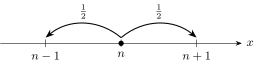
A drunk man is walking along the integer line. He starts at the origin, $X_0 = 0$ . At each step, independently of everything before, he moves one unit right with probability $\tfrac12$ or one unit left with probability $\tfrac12$ . Let $X_n$ be his location after $n$ steps.

Number line with the walker at n and arrows to n − 1 and n + 1, each labeled probability 1/2

Questions: What is $\EE[X_n]$ ? What is $\EE[X_n^2]$ , and how far from the origin is he typically?

Write the $(n+1)$ -th step using two indicator random variables,

\mathbf{1}_{+}^{(n+1)} = \begin{cases} 1 & \text{if step } n+1 \text{ is } +1, \\ 0 & \text{otherwise,} \end{cases} \qquad \mathbf{1}_{-}^{(n+1)} = \begin{cases} 1 & \text{if step } n+1 \text{ is } -1, \\ 0 & \text{otherwise.} \end{cases}

Exactly one of them equals $1$ , so the step is $\mathbf{1}_{+}^{(n+1)} - \mathbf{1}_{-}^{(n+1)} \in \{+1, -1\}$ , and

X_{n+1} = X_n + \mathbf{1}_{+}^{(n+1)} - \mathbf{1}_{-}^{(n+1)}. \tag{5.19}

Notation. An indicator only takes the values $0$ and $1$ , so a step of $-1$ is written by subtracting the indicator $\mathbf{1}_{-}^{(n+1)}$ . The superscript $(n+1)$ records that each step is a fresh, independent coin flip. Similarly, the location $X_n$ and the step taken at time $n$ are different random variables, so we keep separate names for them.

The mean: 𝔼[Xₙ] = 0 for all n

Take expectations in (5.19). By linearity, and since $\EE[\mathbf{1}_{\pm}^{(n+1)}] = \PP(\text{step is } \pm 1) = \tfrac12$ ,

\EE[X_{n+1}] = \EE[X_n] + \EE\bigl[\mathbf{1}_{+}^{(n+1)}\bigr] - \EE\bigl[\mathbf{1}_{-}^{(n+1)}\bigr] = \EE[X_n] + \tfrac12 - \tfrac12 = \EE[X_n]. \tag{5.20}

So one step never changes the expected location.

Theorem 5.3 (Mean of the symmetric random walk)

For every $n \ge 0$ , $\EE[X_n] = 0$ .

Proof.

By induction on $n$ . Base case: $X_0 = 0$ is a constant, so $\EE[X_0] = 0$ . Inductive step: suppose $\EE[X_n] = 0$ . By (5.20), $\EE[X_{n+1}] = \EE[X_n] = 0$ . Unrolled, this is just a chain of equalities:

\EE[X_n] = \EE[X_{n-1}] = \EE[X_{n-2}] = \cdots = \EE[X_1] = \EE[X_0] = 0.

Two more ways to see it.

Sum of steps. Let $\xi_i \in \{+1, -1\}$ be the $i$ -th step, so $X_n = \xi_1 + \xi_2 + \cdots + \xi_n$ . Each step has mean $\EE[\xi_i] = (+1)\cdot\tfrac12 + (-1)\cdot\tfrac12 = 0$ , and by linearity $\EE[X_n] = \sum_{i=1}^n \EE[\xi_i] = 0$ .
Symmetry. Flipping the direction of every step turns the walk $X_n$ into $-X_n$ , and since left and right are equally likely, the flipped walk has exactly the same distribution. So $\EE[X_n] = \EE[-X_n] = -\EE[X_n]$ , which forces $\EE[X_n] = 0$ .

A zero mean does not mean the walker stays near the origin. He drifts away, but is equally likely to drift left or right, so the drifts cancel in the average. To measure how far he wanders, we need the second moment.

The second moment: 𝔼[Xₙ²] = n

Suppose $X_n = k$ . The next step is $\pm 1$ with probability $\tfrac12$ each, independent of the past, so

\PP\bigl(X_{n+1}^2 = (k+1)^2 \mid X_n = k\bigr) = \tfrac12, \qquad \PP\bigl(X_{n+1}^2 = (k-1)^2 \mid X_n = k\bigr) = \tfrac12.

These are the same two equally likely moves ( $k \to k+1$ and $k \to k-1$ ), just with the resulting location squared. Therefore

\begin{aligned} \EE\bigl[X_{n+1}^2 \mid X_n = k\bigr] &= \tfrac12 (k+1)^2 + \tfrac12 (k-1)^2 \\ &= \tfrac12 (k^2 + 2k + 1) + \tfrac12 (k^2 - 2k + 1) \\ &= k^2 + 1. \end{aligned}

The edge case $k = 0$ . When $k = 0$ , $(k+1)^2 = (k-1)^2 = 1$ , so the two events above are the same event, which has probability $1$ (not $\tfrac12$ ). The computation of $\EE[X_{n+1}^2 \mid X_n = 0]$ is still correct, because we are really averaging over the two moves: $\tfrac12 \cdot 1 + \tfrac12 \cdot 1 = 1 = 0^2 + 1$ .

We found $g(k) = \EE[X_{n+1}^2 \mid X_n = k] = k^2 + 1$ . Replacing the value $k$ by the random variable $X_n$ (the “pattern matching” step, exactly as in $\EE[X \mid N] = N/2$ ):

\EE\bigl[X_{n+1}^2 \mid X_n\bigr] = X_n^2 + 1.

By the law of iterated expectation,

\begin{aligned} \EE\bigl[X_{n+1}^2\bigr] &= \EE\bigl[\EE[X_{n+1}^2 \mid X_n]\bigr] && \text{(law of iterated expectation)} \\ &= \EE\bigl[X_n^2 + 1\bigr] \\ &= 1 + \EE\bigl[X_n^2\bigr]. && \text{(linearity)} \end{aligned}

Each step adds exactly $1$ to the second moment, starting from $\EE[X_0^2] = 0$ :

\EE[X_0^2] = 0, \quad \EE[X_1^2] = 1, \quad \EE[X_2^2] = 2, \quad \ldots \quad\Longrightarrow\quad \EE[X_n^2] = n,

(formally, by induction exactly as for the mean). In particular $\EE[X_{n+1}^2] = 1 + n$ .

Theorem 5.4 (Spread of the symmetric random walk)

For every $n \ge 0$ ,

\Var(X_n) = \EE[X_n^2] - (\EE[X_n])^2 = n - 0^2 = n, \qquad\text{so}\qquad \sigma_{X_n} = \sqrt{n}.

Cross-check with Lecture 4. With $X_n = \xi_1 + \cdots + \xi_n$ and independent steps, each step has $\Var(\xi_i) = \EE[\xi_i^2] - 0^2 = 1$ (since $\xi_i^2 = 1$ always). The variance of a sum of independent random variables is the sum of the variances, so $\Var(X_n) = n$ . Same answer, no conditioning needed.

Key takeaway. The walker’s expected position is $0$ forever, but his typical distance from the origin is $\sqrt{n}$ : after $10{,}000$ steps he is typically about $100$ units away. This $\sqrt{n}$ growth is the signature of diffusion, and it reappears throughout the course.

Conditional Variance and the Law of Total Variance

Definition 5.1 (Conditional variance)

For $y$ with $\PP(Y = y) > 0$ , the conditional variance of $X$ given $Y = y$ is the variance of the conditional distribution of $X$ :

\Var(X \mid Y = y) \triangleq \EE\Bigl[\bigl(X - \EE[X \mid Y = y]\bigr)^2 \Bigm| Y = y\Bigr] = \EE[X^2 \mid Y = y] - \bigl(\EE[X \mid Y = y]\bigr)^2.

This is a number for each $y$ , so $\Var(X \mid Y)$ , obtained by replacing $y$ with $Y$ , is a function of $Y$ , and hence a random variable.

(The second form follows exactly as in Lecture 3, applied to the conditional distribution of $X$ given $Y = y$ .)

Theorem 5.5 (Law of total variance)

For random variables $X, Y$ with $\EE[X^2] < \infty$ ,

\Var(X) = \EE\bigl[\Var(X \mid Y)\bigr] + \Var\bigl(\EE[X \mid Y]\bigr).

Proof.

Abbreviate $\mu(Y) = \EE[X \mid Y]$ , so that $\Var(X \mid Y) = \EE[X^2 \mid Y] - \mu(Y)^2$ .

Take expectations and use the tower rule on $\EE[X^2 \mid Y]$ :

\EE\bigl[\Var(X \mid Y)\bigr] = \EE\bigl[\EE[X^2 \mid Y]\bigr] - \EE\bigl[\mu(Y)^2\bigr] = \EE[X^2] - \EE\bigl[\mu(Y)^2\bigr].

Next, $\mu(Y)$ is a random variable; apply the variance formula to it, and use the tower rule on its mean, $\EE[\mu(Y)] = \EE[\EE[X\mid Y]] = \EE[X]$ :

\Var\bigl(\mu(Y)\bigr) = \EE\bigl[\mu(Y)^2\bigr] - \bigl(\EE[\mu(Y)]\bigr)^2 = \EE\bigl[\mu(Y)^2\bigr] - (\EE[X])^2.

Adding the two, the $\EE[\mu(Y)^2]$ terms cancel:

\begin{aligned} \EE\bigl[\Var(X \mid Y)\bigr] + \Var\bigl(\EE[X \mid Y]\bigr) &= \EE[X^2] - \EE\bigl[\mu(Y)^2\bigr] + \EE\bigl[\mu(Y)^2\bigr] - (\EE[X])^2 \\ &= \Var(X). \end{aligned}

Interpretation: within-group plus between-group. Group the outcomes by the value of $Y$ . Then $\EE[\Var(X \mid Y)]$ is the average spread within each group, and $\Var(\EE[X \mid Y])$ is the spread between the group means. Total spread is the sum of the two. Since both terms are nonnegative, $\Var(X) \ge \EE[\Var(X \mid Y)]$ : on average, learning $Y$ can only reduce our uncertainty about $X$ .

Example 5.5 (Variance of heads in a random number of tosses)

Continue the example with $N \sim \Geom(p)$ and $X \mid N \sim \Bin(N, \tfrac12)$ . From the binomial formulas of Lecture 4,

\EE[X \mid N] = \frac{N}{2}, \qquad \Var(X \mid N) = N \cdot \tfrac12 \cdot \tfrac12 = \frac{N}{4}.

Using $\EE[N] = \frac1p$ and $\Var(N) = \frac{1-p}{p^2}$ :

\begin{aligned} \EE\bigl[\Var(X \mid N)\bigr] &= \EE\Bigl[\frac{N}{4}\Bigr] = \frac14 \cdot \frac1p = \frac{1}{4p}, \\ \Var\bigl(\EE[X \mid N]\bigr) &= \Var\Bigl(\frac{N}{2}\Bigr) = \frac14\,\Var(N) = \frac{1-p}{4p^2}. \end{aligned}

By the law of total variance,

\Var(X) = \frac{1}{4p} + \frac{1-p}{4p^2} = \frac{p}{4p^2} + \frac{1-p}{4p^2} = \frac{1}{4p^2}.

Sanity check: if $p = 1$ , then $N = 1$ and $X \sim \Bern(\tfrac12)$ , whose variance is $\tfrac12\cdot\tfrac12 = \tfrac14$ . ✓

Continuous Random Variables

Continuous random variables (CRVs) let us measure uncertainty in a principled way for quantities that vary continuously, such as velocity, time, and distance.

Coming up. Important continuous distributions include the uniform, exponential, and gamma distributions, which we develop in upcoming lectures. The exponential is the continuous analog of the geometric (Lecture 4).

Why discrete tools break. Let $X \sim \operatorname{Uniform}[0,1]$ , a number chosen “uniformly at random” from $[0,1]$ . Then:

$\PP(X = x) = 0$ for any specific number $x$ (there are uncountably many equally likely candidates);
yet $\PP(X < \tfrac12) = \tfrac12$ .

So we cannot build probabilities by adding up point masses as we did with PMFs. Instead, we assign probabilities directly to sets that are “allowable events.”

Definition 5.2 (Allowable events (Borel sets))

The allowable events for a real-valued random variable include all intervals,

(-\infty, a), \qquad [a, b], \qquad (a, b], \qquad \ldots

together with everything obtainable from intervals by countable unions, countable intersections, and complements, e.g. $(a, b) \cup (c, d)$ . These are the Borel sets; they form the Borel $\sigma$ -algebra from Lecture 1. In practice, any “reasonable” set is allowable.

Recall that for a discrete random variable (DRV) and a set of values $B$ ,

\PP(X \in B) = \sum_{x \in B} p_X(x).

For a CRV, the sum over points becomes an integral of a density.

Definition 5.3 (Continuous random variable and PDF)

A random variable $X$ is continuous if there is a function $f_X : \RR \to [0, \infty)$ , called its probability density function (PDF), such that for every allowable set $B$ ,

\PP(X \in B) = \int_B f_X(x)\,dx.

A density must satisfy

f_X(x) \ge 0 \;\text{ for all } x, \qquad\text{and}\qquad \int_{-\infty}^{\infty} f_X(x)\,dx = 1.

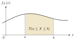
In particular, $\PP(a \le X \le b) = \int_a^b f_X(x)\,dx$ is the area under the density between $a$ and $b$ .

A density curve f_X(x) with the area between a and b shaded, labeled P(a ≤ X ≤ b)

Theorem 5.6 (Single points have probability zero)

If $X$ is continuous, then $\PP(X = x) = 0$ for every $x \in \RR$ .

Proof.

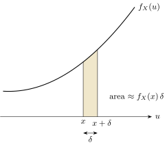
Fix $x$ and any $\delta > 0$ . The event $\{X = x\}$ is contained in $\{x \le X < x + \delta\}$ , so

\PP(X = x) \le \PP(x \le X < x + \delta) = \int_x^{x+\delta} f_X(u)\,du.

(We use the dummy variable $u$ inside the integral so as not to confuse it with $x$ , which now appears in the limits.) As $\delta \to 0$ , this is the integral of $f_X$ over a shrinking interval, which tends to $0$ . If $f_X$ is continuous at $x$ , we can see this explicitly: the sliver is approximately a rectangle of height $f_X(x)$ and width $\delta$ , so the integral is $\approx f_X(x)\,\delta \to 0$ . Since $\PP(X = x)$ is smaller than a quantity that can be made arbitrarily small, $\PP(X = x) = 0$ .

A thin sliver under the density f_X(u) between x and x + δ, with area approximately f_X(x) δ

A density is not a probability. $f_X(x)$ has units of probability per unit length. Wherever $f_X$ is continuous,

f_X(x) = \lim_{\delta \to 0} \frac{\PP(x \le X < x + \delta)}{\delta}, \quad\text{i.e.}\quad \PP(x \le X < x + \delta) \approx f_X(x)\,\delta \text{ for small } \delta.

Don’t confuse $f_X(x)$ with a probability: it is a density. Only areas under $f_X$ are probabilities, so $f_X(x)$ itself may exceed $1$ , as the next example shows.

Example 5.6 (An unbounded density)

Let

f_X(x) = \begin{cases} \dfrac{1}{2\sqrt{x}} & 0 < x \le 1, \\[4pt] 0 & \text{otherwise.} \end{cases}

It is a valid PDF. Clearly $f_X \ge 0$ . For the total area, write $\frac{1}{2\sqrt{x}} = \frac12 x^{-1/2}$ and integrate:

\int_{-\infty}^{\infty} f_X(x)\,dx = \int_0^1 \tfrac12\, x^{-1/2}\,dx = \tfrac12 \Bigl[\, 2x^{1/2} \Bigr]_0^1 = \Bigl[\sqrt{x}\,\Bigr]_0^1 = 1 - 0 = 1.

It exceeds $1$ , and is even unbounded. $f_X(1) = \tfrac12$ , but $f_X(0.01) = \frac{1}{2(0.1)} = 5$ , and $f_X(x) \to \infty$ as $x \to 0^+$ . Nevertheless every probability is finite, e.g. $\PP(X \le 0.01) = \int_0^{0.01}\tfrac12 x^{-1/2}\,dx = \sqrt{0.01} = 0.1$ .

Graph of f_X(x) = 1/(2√x) on (0, 1], rising without bound as x approaches 0, with the area underneath shaded

The Cumulative Distribution Function

Definition 5.4 (Cumulative distribution function (CDF))

The cumulative distribution function of any random variable $X$ (discrete or continuous) is

F_X(x) \triangleq \PP(X \le x), \qquad x \in \RR.

For a continuous random variable,

F_X(x) = \int_{-\infty}^{x} f_X(u)\,du.

Theorem 5.7 (Properties of the CDF)

Every CDF satisfies:

Nondecreasing: if $x \le y$ then $F_X(x) \le F_X(y)$ , since $\{X \le x\} \subseteq \{X \le y\}$ .
Limits: $\displaystyle\lim_{x \to -\infty} F_X(x) = 0$ and $\displaystyle\lim_{x \to +\infty} F_X(x) = 1$ .
Intervals: $\PP(a < X \le b) = F_X(b) - F_X(a)$ , because $\{X \le b\}$ is the disjoint union of $\{X \le a\}$ and $\{a < X \le b\}$ .

Theorem 5.8 (Recovering the PMF or PDF from the CDF)

CRV: wherever $f_X$ is continuous, $f_X(x) = \frac{dF_X(x)}{dx}.$
Integer-valued DRV: for every integer $k$ , $\PP(X = k) = F_X(k) - F_X(k-1).$

Proof.

CRV: $F_X(x) = \int_{-\infty}^x f_X(u)\,du$ , so this is the fundamental theorem of calculus. DRV: because $X$ only takes integer values, there are no possible values strictly between $k-1$ and $k$ . So $\{X \le k\}$ is the disjoint union of $\{X \le k-1\}$ and $\{X = k\}$ , giving $F_X(k) = F_X(k-1) + \PP(X = k)$ . (For a discrete random variable taking non-integer values, use the jump of $F_X$ at the value instead.)

Picturing the two kinds of CDF. For an integer-valued DRV, $F_X$ is a staircase. On each open interval $(k-1, k)$ there are no possible values, so no new probability accumulates and $F_X$ stays flat, holding the value $F_X(k-1)$ . It does not drop back to zero: all the probability collected up through $k-1$ is still counted. At $k$ itself, $F_X$ jumps up by exactly $\PP(X = k)$ . For a CRV, single points carry no probability, so $F_X$ rises continuously with no jumps.

Left: the staircase CDF of an integer-valued discrete random variable, jumping by P(X = k) at k. Right: the continuous CDF of Uniform[0,1], rising linearly from 0 to 1

Corollary 5.1 (Consequences for continuous random variables)

If $X$ is continuous, then for all $a \le b$ :

\PP(a \le X \le b) = \int_a^b f_X(x)\,dx = F_X(b) - F_X(a),

\PP(X = a) = 0, \qquad \PP(X < a) = \PP(X \le a).

Because points do not contribute, it does not matter whether the endpoints of an interval are included: $\PP(a < X < b) = \PP(a \le X < b) = \PP(a < X \le b) = \PP(a \le X \le b)$ . This is false for discrete random variables, where $\PP(X < k)$ and $\PP(X \le k)$ differ by $\PP(X = k)$ .

Example: A Random Dart on a Disk

Example 5.7 (Random dart on the unit disk)

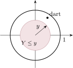
A dart lands uniformly at random on a disk of radius $1$ (the unit circle and its interior). “Uniformly” means the probability of landing in any region is proportional to its area:

\PP(\text{dart lands in region } R) = \frac{\text{Area}(R)}{\text{Area of full disk}} = \frac{\text{Area}(R)}{\pi (1)^2}.

Let $Y$ be the dart’s distance from the center. Find the PDF $f_Y(y)$ .

Unit disk with a shaded inner disk of radius y, labeled Y ≤ y, and a dart landing inside the unit disk

It is easiest to compute $F_Y(y) = \PP(Y \le y)$ first. For $0 \le y \le 1$ , the event $\{Y \le y\}$ means the dart lands in the shaded disk of radius $y$ :

F_Y(y) = \PP(Y \le y) = \frac{\text{Area shaded}}{\text{Area full disk}} = \frac{\pi y^2}{\pi (1)^2} = y^2.

Outside $[0,1]$ : $F_Y(y) = 0$ for $y < 0$ (distance is never negative) and $F_Y(y) = 1$ for $y > 1$ (the dart is always on the disk).

Differentiating,

f_Y(y) = \frac{dF_Y(y)}{dy} = \frac{d}{dy}\bigl(y^2\bigr) = 2y, \qquad 0 \le y \le 1,

and $f_Y(y) = 0$ otherwise. Check: $\int_0^1 2y\,dy = \bigl[y^2\bigr]_0^1 = 1$ . ✓

By the CDF,

\PP\bigl(Y \in (0.5, 0.6)\bigr) = F_Y(0.6) - F_Y(0.5) = 0.6^2 - 0.5^2 = 0.36 - 0.25 = 0.11.

Or, equivalently, by the PDF: $\int_{0.5}^{0.6} 2y\,dy = \bigl[y^2\bigr]_{0.5}^{0.6} = 0.11$ .

Three traps in this example.

$Y$ is not uniform on $[0,1]$ . The dart’s position is uniform on the disk, but its distance from the center is not: the density $2y$ grows with $y$ , because there is more area at larger radii. The ring $0.5 < Y < 0.6$ has probability $0.11$ , while the same-width band $0 < Y < 0.1$ near the center has only $0.1^2 = 0.01$ .
Don’t stop at the CDF. $y^2$ is $F_Y$ , not $f_Y$ ; the PDF requires the extra differentiation step.
$\frac{1}{\pi r^2}$ is a 2-D density. The constant $\frac{1}{\pi r^2}$ (here $\frac1\pi$ ) is the density of the dart’s position per unit area. It is not $f_Y$ , which is a density per unit length along the radius.

The CDF method. This “CDF first, then differentiate” strategy is the standard way to find the density of a function of a random variable.

Example: Meeting at Random Times

Not finished in lecture. We ran out of time after posing this problem. The full solution is given below.

Example 5.8 (Will A and B meet?)

$A$ and $B$ each arrive at a meeting spot at a uniformly random time between 4:00 pm and 5:00 pm, independently of each other. Whoever arrives first waits $10$ minutes and then leaves. What is $\PP(A \text{ and } B \text{ meet})$ ?

Setup. Measure time in minutes after 4:00 pm, so $A$ and $B$ are independent $\operatorname{Uniform}[0, 60]$ random variables. The pair $(A, B)$ is a point in the $60 \times 60$ square $[0,60]^2$ . Because $A$ and $B$ are independent and each uniform, the point $(A, B)$ is uniform on the square:

\PP\bigl((A, B) \in R\bigr) = \frac{\text{Area}(R)}{60 \times 60} = \frac{\text{Area}(R)}{3600}.

(Joint distributions of several continuous random variables are developed formally in upcoming lectures; this “probability $=$ area fraction” rule is the two-dimensional version of the uniform distribution, exactly as in the dart example.)

When do they meet? Whoever arrives first waits $10$ minutes, so they meet exactly when their arrival times differ by at most $10$ minutes:

\{A \text{ and } B \text{ meet}\} = \bigl\{|A - B| \le 10\bigr\}.

This is the shaded diagonal band in the figure below.

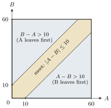
The 60 by 60 square of arrival times (A, B), with the diagonal band |A − B| ≤ 10 shaded as the meeting region and two corner triangles where they miss each other

Compute the complement. The two blue corner regions, where they miss each other, are right triangles:

$\{A - B > 10\}$ : $A$ arrives more than $10$ minutes after $B$ , so $B$ has already left. The triangle has vertices $(10,0), (60,0), (60,50)$ and legs of length $50$ .
$\{B - A > 10\}$ : the mirror image, with vertices $(0,10), (0,60), (50,60)$ , also with legs of length $50$ .

Each triangle has area $\tfrac12 \cdot 50 \cdot 50 = 1250$ , so together they cover $2500$ out of $3600$ :

\PP(\text{miss}) = \frac{2 \cdot 1250}{3600} = \frac{2500}{3600} = \frac{25}{36}.

Therefore

\PP(A \text{ and } B \text{ meet}) = 1 - \frac{25}{36} = \frac{11}{36} \approx 0.306.

Equivalently, the band has area $3600 - 2500 = 1100$ , and $\frac{1100}{3600} = \frac{11}{36}$ .

Checks and generalization.

Boundaries don’t matter. The lines $|A - B| = 10$ have zero area, so it makes no difference whether “waits $10$ minutes” includes the endpoint. This is the two-dimensional version of $\PP(X < a) = \PP(X \le a)$ .
General formula. With a window of length $T$ and waiting time $w \le T$ , the same picture gives $\PP(\text{meet}) = 1 - \Bigl(1 - \frac{w}{T}\Bigr)^2.$ With $w = 10$ , $T = 60$ : $1 - (5/6)^2 = 11/36$ . Sanity checks: $w = 0$ gives $0$ (they must arrive at the exact same instant), and $w = T$ gives $1$ .

iterated-expectation-and-continuous-random-variables.html

Lecture 5: Iterated Expectation, Conditional Variance, and Continuous Random Variables

The St. Petersburg Paradox

Conditional Expectation as a Random Variable

The Law of Iterated Expectation (Tower Property)

The Symmetric Random Walk

The mean: 𝔼[Xₙ] = 0 for all n

The second moment: 𝔼[Xₙ²] = n

Conditional Variance and the Law of Total Variance

Continuous Random Variables

The Cumulative Distribution Function

Example: A Random Dart on a Disk

Example: Meeting at Random Times