These are my personal notes from Professor Kannan Ramchandran’s EECS 126 (Probability and Random Processes) course at UC Berkeley.
Last lecture we defined expectation and variance for a single random variable. In this lecture we study how variance behaves for sums of random variables, which leads to covariance and the correlation coefficient. We then compute the mean and variance of the four workhorse discrete distributions (Bernoulli, binomial, geometric, Poisson), apply these to the coupon collector problem, prove the memoryless property of the geometric distribution, study how Poisson random variables merge and split, and finally introduce conditional expectation.
Variance of Sums and Covariance
Recall from Lecture 3 the two forms of the variance,
Var(X)=E[(X−E[X])2]=E[X2]−(E[X])2,
and the scaling property
Var(aX+c)=a2Var(X).
Shifts by a constant c are not recorded in variance calculations: shifting every outcome by c moves the mean by c as well, so the deviations X−E[X] are unchanged.
The natural next question is: what is the variance of a sumX+Y? Unlike the mean, the answer depends on how X and Y interact.
Theorem 4.1 (Variance of a sum)
For any random variables X,Y with finite variances,
No independence was used. The derivation above holds for anyX and Y. Independence only enters at the very end, where it makes the cross term vanish (Corollary 4.1 below).
The cross term in (4.3) is important enough to get its own name.
Definition 4.1 (Covariance)
The covariance of random variables X and Y is
Cov(X,Y)≜E[(X−E[X])(Y−E[Y])]=E[XY]−E[X]E[Y].
In particular, Cov(X,X)=Var(X). With this notation,
Var(X+Y)=Var(X)+Var(Y)+2Cov(X,Y).
Equivalence of the two forms.
Write μX=E[X] and μY=E[Y], which are constants. Expanding the product and using linearity,
Interpreting the sign.Cov(X,Y)>0 means X and Y tend to be above their means together (and below their means together). Cov(X,Y)<0 means when one is above its mean, the other tends to be below. For a sum, positive covariance inflates the spread and negative covariance dampens it.
Corollary 4.1 (Independent summands)
If X⊥Y, then Cov(X,Y)=0, and therefore
Var(X+Y)=Var(X)+Var(Y).
Proof.
In Lecture 3 we proved that X⊥Y implies E[XY]=E[X]E[Y]. Hence Cov(X,Y)=E[XY]−E[X]E[Y]=0, and the cross term in (4.3) vanishes.
Corollary 4.2 (Variance of a sum of many random variables)
For random variables X1,…,Xn with finite variances,
Var(i=1∑nXi)=i=1∑nVar(Xi)+2i<j∑Cov(Xi,Xj).
In particular, if the Xi are independent (in fact, pairwise uncorrelated is enough), then
Var(i=1∑nXi)=i=1∑nVar(Xi).
Proof.
Let μi=E[Xi]. Since E[∑iXi]=∑iμi, the centered sum is ∑i(Xi−μi). Squaring a sum gives a double sum over all pairs (i,j):
The diagonal terms i=j give Cov(Xi,Xi)=Var(Xi). The off-diagonal terms come in symmetric pairs, Cov(Xi,Xj)=Cov(Xj,Xi), so they contribute 2∑i<jCov(Xi,Xj). If every pair is uncorrelated, all off-diagonal terms are zero.
Uncorrelated does not imply independent. Covariance only detects linear dependence. For example, let X be uniform on {−1,0,1} and Y=X2. Then E[X]=0 and E[XY]=E[X3]=31(−1)+31(0)+31(1)=0, so Cov(X,Y)=0−0⋅E[Y]=0. But Y is completely determined by X: for instance P(Y=0∣X=0)=1=31=P(Y=0). This was a question Ramchandran asked us at end of previous lecture.
The Correlation Coefficient
Covariance has units (units of X times units of Y), so its size alone does not tell us how strongly two variables are related. Normalizing by the standard deviations removes the units.
Definition 4.2 (Correlation coefficient)
For random variables X,Y with Var(X)>0 and Var(Y)>0, the correlation coefficient is
ρ(X,Y)≜Var(X)Var(Y)Cov(X,Y).
Ramchandran’s vector analogy. Think of random variables as vectors, with “dot product” ⟨U,V⟩=E[UV] and “length” E[U2]. For the centered variables U=X−E[X] and V=Y−E[Y]:
the dot product is E[UV]=Cov(X,Y);
the lengths are E[U2]=Var(X) and E[V2]=Var(Y).
So ρ plays the role of cosθ=∣u∣∣v∣u⋅v, the cosine of the angle between two vectors. For ordinary vectors, the Cauchy–Schwarz inequality ∣u⋅v∣≤∣u∣∣v∣ forces −1≤cosθ≤1. The same inequality, proved for random variables below, forces −1≤ρ≤1.
Lemma 4.1 (Cauchy–Schwarz inequality for random variables)
For any random variables U,V with E[U2]<∞ and E[V2]<∞,
(E[UV])2≤E[U2]E[V2].
Proof.
Case 1: E[V2]=0. Since V2≥0 and its mean is 0, we must have V=0 with probability 1. Then UV=0 with probability 1, so E[UV]=0 and both sides equal 0.
Case 2: E[V2]>0. For every real number t, the random variable (U−tV)2 is nonnegative, so its expectation is nonnegative. Expanding with linearity:
0≤E[(U−tV)2]=E[U2]−2tE[UV]+t2E[V2].
This holds for every t, so choose the t that minimizes the right-hand side, namely t⋆=E[UV]/E[V2]. Substituting,
Multiplying both sides by E[V2]>0 gives (E[UV])2≤E[U2]E[V2].
Theorem 4.2 (Range of the correlation coefficient)
Whenever ρ(X,Y) is defined,
−1≤ρ(X,Y)≤1.
Proof.
Apply Cauchy–Schwarz to the centered variables U=X−E[X] and V=Y−E[Y]. By definition, E[UV]=Cov(X,Y), E[U2]=Var(X), and E[V2]=Var(Y), so
(Cov(X,Y))2≤Var(X)Var(Y).
Taking square roots, ∣Cov(X,Y)∣≤Var(X)Var(Y). Dividing by the (positive) right-hand side gives ∣ρ(X,Y)∣≤1.
Extreme and zero values.∣ρ∣=1 exactly when equality holds in Cauchy–Schwarz, which happens when U−t⋆V=0 with probability 1, i.e. when Y is an exact linear function Y=aX+b of X (with ρ=+1 if a>0 and ρ=−1 if a<0). At the other end, ρ=0 means uncorrelated, which, as we just saw, is weaker than independent.
Mean and Variance of Common Distributions
We now compute E[X] and Var(X) for the four distributions introduced in Lecture 3. A recurring theme: the direct sums are often messy, and a better representation of the random variable makes the computation easy.
Bernoulli
Theorem 4.3 (Bernoulli mean and variance)
If X∼Bernoulli(p), then
E[X]=p,Var(X)=p(1−p).
Proof.
X takes only the values 0 and 1, with P(X=1)=p and P(X=0)=1−p.
E[X]=1⋅P(X=1)+0⋅P(X=0)=1⋅p+0=p.
For the second moment, by LOTUS,
E[X2]=x∑x2P(X=x)=12⋅P(X=1)+02⋅P(X=0)=p.
Therefore
Var(X)=E[X2]−(E[X])2=p−p2=p(1−p).
Binomial
Theorem 4.4 (Binomial mean and variance)
If X∼Binomial(n,p), then
E[X]=np,Var(X)=np(1−p).
The direct approach is
E[X]=x=0∑nx⋅P(X=x)=x=0∑nx(xn)px(1−p)n−x,
which is doable but unpleasant. Instead, think of the binomial as a sum of n Bernoulli trials.
Proof.
Let Xi=1{trial i is a success} for i=1,…,n. Each Xi∼Bernoulli(p), the Xi are independent (the trials are independent), and the total number of successes is
X=X1+X2+⋯+Xn.
Mean. By linearity of expectation (which needs no independence),
E[X]=i=1∑nE[Xi]=i=1∑np=np.
Variance. Because the Xi are independent, Corollary 4.2 lets us add the variances:
Var(X)=i=1∑nVar(Xi)=i=1∑np(1−p)=np(1−p).
Applying direct sum gives us the same result: Using the identity x(xn)=n(x−1n−1) for x≥1 (the x=0 term is zero),
where we substituted j=x−1 and used the binomial theorem. The indicator method reaches the same answer with far less algebra.
Geometric
Recall that X∼Geometric(p) counts the number of independent trials up to and including the first success:
pX(k)=P(X=k)=(1−p)k−1p,k=1,2,3,…
Reading the PMF. Here k marks the trial on which the first Success occurs (k=S). So pX(k) is the probability that the first success happens on trial k: the first k−1 trials are failures (probability (1−p)k−1) and trial k is a success (probability p). Note that pX(k) is not the probability of k successes; a geometric random variable always records exactly one success, and k counts how long we waited for it.
Definition 4.3 (Survival function)
For an integer-valued random variable X, the survival function (or tail) is k↦P(X>k). For X∼Geometric(p),
P(X>k)=(1−p)k,k=0,1,2,…(4.27)
Proof.
The event {X>k} means “no success in the first k trials,” i.e. we tried k times and failed every time. The trials are independent and each fails with probability 1−p, so P(X>k)=k times(1−p)⋯(1−p)=(1−p)k.
Theorem 4.5 (Geometric mean)
If X∼Geometric(p) with 0<p≤1, then
E[X]=p1.
The direct sum E[X]=∑k=1∞k(1−p)k−1p requires a trick. A better method is the tail sum formula from Lecture 3, which applies because X takes values in the nonnegative integers.
Proof.
By the tail sum formula,
E[X]=k=1∑∞P(X≥k).
For integer-valued X, {X≥k}={X>k−1}. Substituting j=k−1 (so j runs from 0 to ∞),
E[X]=k=1∑∞P(X>k−1)=j=0∑∞P(X>j).
Now plug in the survival function (4.27):
E[X]=j=0∑∞(1−p)j.
This is a geometric series ∑j≥0xj with ratio x=1−p. Since 0<p≤1 we have ∣x∣<1, so the series converges to 1/(1−x):
E[X]=1−(1−p)1=p1.
Exam note: tail sum formula will be on exam. For a random variable X taking values in {0,1,2,…},
E[X]=k=1∑∞P(X≥k)=k=0∑∞P(X>k).
It expresses the mean as the sum of the tail probabilities. It follows from writing X=∑k=1∞1{X≥k} and taking expectations of both sides.
The direct sum, for comparison. Differentiating the geometric series ∑k≥0xk=1−x1 term by term (valid for ∣x∣<1) gives ∑k≥1kxk−1=(1−x)21. With x=1−p,
E[X]=pk=1∑∞k(1−p)k−1=p⋅(1−(1−p))21=p⋅p21=p1.
The variance of the geometric is derived in Section 4.5, using the memoryless property.
Poisson
Theorem 4.6 (Poisson mean and variance)
If X∼Poisson(λ), so that pX(k)=k!e−λλk for k=0,1,2,…, then
E[X]=λ,Var(X)=λ.
Both computations rely on the Taylor series of the exponential,
ex=i=0∑∞i!xi=1+x+2!x2+3!x3+⋯,(4.36)
and on the cancellation k!k=(k−1)!1 for k≥1.
Proof of the mean.E[X]=k=0∑∞k⋅k!e−λλk=k=1∑∞k⋅k!e−λλk=k=1∑∞(k−1)!e−λλk=λe−λk=1∑∞(k−1)!λk−1=λe−λj=0∑∞j!λj=λe−λeλ=λ.(the k=0 term is 0)(cancel k against k!)(factor out λe−λ)(substitute j=k−1)(Taylor series (4.36))
For the variance, computing E[X2]=∑k2k!e−λλk directly is awkward because k2 does not cancel cleanly against k!. The fix is the factorial moment trick: since X2=X(X−1)+X, linearity gives
E[X2]=E[X(X−1)]+E[X],(4.37)
and k(k−1) cancels against k! just as k did.
Proof of the variance.
Step 1: the factorial moment.
E[X(X−1)]=k=0∑∞k(k−1)k!e−λλk=k=2∑∞k(k−1)k!e−λλk=k=2∑∞(k−2)!e−λλk=e−λλ2k=2∑∞(k−2)!λk−2=e−λλ2eλ=λ2.(the k=0,1 terms are 0)(cancel k(k−1) against k!)(factor out e−λλ2)(same trick: substitute j=k−2)
Step 2: the second moment. By (4.37),
E[X2]=E[X(X−1)]+E[X]=λ2+λ.
Step 3: the variance.
Var(X)=E[X2]−(E[X])2=(λ2+λ)−(λ)2=λ.
Mean equals variance (Poisson distribution). The Poisson is the only one of our four distributions whose mean and variance are equal. This is consistent with the Poisson being the limit of Binomial(n,λ/n): the binomial variance is n⋅nλ(1−nλ)=λ(1−nλ)→λ as n→∞.
The Coupon Collector Problem
Example 4.1 (Coupon collector)
There are N different coupons you want to collect, found inside cereal boxes. Each box contains exactly one coupon, whose type is uniformly random among the N types and independent of all other boxes. You buy boxes until you have received all N distinct coupons. What is the expected number of boxes you must buy?
Let T be the total time (number of boxes) to collect all N coupons. Break the process into N stages. For i=1,…,N, let
Ti=# of boxes bought to obtain the i-th new coupon,
counting from right after the (i−1)-th new coupon was obtained. Then the total time is the sum of the stage times,
T=i=1∑NTi.
Each stage is geometric. During stage i we already hold i−1 distinct coupons, so N−(i−1)=N−i+1 types would be new. Each box is independently a “success” (a new type) with probability
pi=NN−i+1,soTi∼Geometric(NN−i+1).
i=1: T1∼Geometric(NN−1+1)=Geometric(1), so T1=1. The first box always gives a new coupon.
i=2: T2∼Geometric(NN−2+1)=Geometric(NN−1).
i=N: TN∼Geometric(N1). The last coupon is the hardest to find.
Expected total. Since E[Ti]=1/pi=N−i+1N, linearity of expectation gives
E[T]=E[i=1∑NTi]=i=1∑NE[Ti]=i=1∑NN−i+1N.
Write out the terms, from i=1 (denominator N) to i=N (denominator 1):
where we substituted j=N−i+1 (as i runs from 1 to N, j runs from N down to 1). The sum is the N-th harmonic numberHN=∑j=1Nj1, so
E[T]=NHN.
Lemma 4.2 (Size of the harmonic numbers)
For every N≥1,
ln(N+1)≤HN≤1+lnN,
and more precisely HN=lnN+γ+o(1), where γ≈0.5772 is the Euler–Mascheroni constant.
Proof of the bounds.
Compare each term 1/j with the area under the curve 1/x. Since 1/x is decreasing, on the interval [j,j+1] we have 1/x≤1/j, and on [j−1,j] we have 1/x≥1/j. Hence
∫jj+1xdx≤j1≤∫j−1jxdx(j≥2 for the right inequality).
Summing the left inequality over j=1,…,N gives HN≥∫1N+1xdx=ln(N+1). Summing the right inequality over j=2,…,N and adding the j=1 term gives HN≤1+∫1Nxdx=1+lnN. (The sharper statement with γ is a classical result we take as given.)
Corollary 4.3 (Coupon collector asymptotics)
E[T]=NHN≈NlnN+γN≈NlnN.
So we need to buy about a factor of lnN more boxes than the N coupons we are trying to collect.
Numbers and intuition. For N=50, H50≈4.499, so E[T]≈225 boxes, about 4.5× the number of coupon types. Most of the cost comes at the end: the final coupon alone takes E[TN]=N boxes on average, while the entire first half of the collection takes fewer than N boxes in total (∑i≤N/2N−i+1N≤2N⋅2=N). This NlnN behavior shows up whenever we need to “hit every bin” by random sampling: hashing, load balancing, and covering every node in a network.
The Memoryless Property
Theorem 4.7 (Memoryless property of the geometric)
Let X∼Geometric(p) with 0<p<1. For all integers s,t≥0,
P(X>s+t∣X>s)=P(X>t).
In words: given that we have already failed s times, the probability of failing t more times is the same as if we were starting over from scratch.
Proof.
First note that P(X>s)=(1−p)s>0, so the conditional probability is well defined. By the definition of conditional probability,
P(X>s+t∣X>s)=P(X>s)P({X>s+t}∩{X>s}).
Since s+t≥s, the event {X>s+t} is contained in {X>s} (if we have s+t failures, we certainly have s failures), so the intersection is just {X>s+t}:
P(X>s+t∣X>s)=P(X>s)P(X>s+t).
Both numerator and denominator are values of the geometric survival function (4.27):
P(X>s)P(X>s+t)=(1−p)s(1−p)s+t=(1−p)t,
which is exactly the survival function of the geometric evaluated at t, i.e. P(X>t).
Two remarks on memorylessness.
The remaining wait is again geometric. Given X>s, the number of additional trials X−s has the same distribution as X: for k≥1,
P(X−s=k∣X>s)=P(X>s)P(X=s+k)=(1−p)s(1−p)s+k−1p=(1−p)k−1p.
This is the form we use in the derivations below.
Uniqueness. The geometric is the only memoryless distribution on {1,2,3,…}. Its continuous analog, the exponential distribution, will be the only memoryless continuous distribution.
To use memorylessness to recompute E[X], we need to split an expectation according to which of several events occurred. This is the expectation version of the law of total probability from Lecture 2.
Theorem 4.8 (Total expectation theorem)
Let A1,…,An be a partition of Ω with P(Ai)>0 for each i, and define the conditional expectation given an event, E[X∣Ai]=∑xxP(X=x∣Ai). Then
E[X]=i=1∑nP(Ai)E[X∣Ai].
Proof.
For each value x, the law of total probability gives P(X=x)=∑iP(Ai)P(X=x∣Ai). Substituting into the definition of expectation and swapping the order of summation (justified by absolute convergence),
Let X∼Geometric(p). Condition on the outcome of the first trial, using the partition {X=1} (first trial succeeds) and {X>1} (first trial fails):
E[X]=P(X=1)E[X∣X=1]+P(X>1)E[X∣X>1].
P(X=1)=p (success on the first try), and then X=1 exactly, so E[X∣X=1]=1.
P(X>1)=1−p. If the first trial failed, the geometric “tells us we start again”: by memorylessness the remaining wait X−1 is again Geometric(p), and we have already spent one trial. So
E[X∣X>1]=E[(X−1)+1∣X>1]=E[X]+1.
Subtracting E[X] from both sides gives 0=1−pE[X], i.e. pE[X]=1, so
E[X]=p1,
matching the tail sum computation.
Two checks on this argument.
Finiteness. Subtracting E[X] from both sides is only legitimate because E[X]<∞, which we already know from the tail sum. (If E[X]=∞, the equation ∞=∞+1−∞ says nothing.)
Sanity check the answer. Any correct formula must satisfy E[X]≥1 (you need at least one trial) and E[X]→∞ as p→0. A sign slip in the algebra can produce E[X]=1+p1, which fails both tests, since it is less than 1 for every p>0.
Theorem 4.9 (Geometric variance (supplementary))
If X∼Geometric(p), then
Var(X)=p21−p.
Proof.
We use the same first-trial conditioning, now on E[X2] (which is finite, since the tail of X decays geometrically).
E[X2]=P(X=1)E[X2∣X=1]+P(X>1)E[X2∣X>1].
Given X=1: X2=1, so E[X2∣X=1]=1.
Given X>1: by memorylessness, X=1+X′ where X′∼Geometric(p) has the same distribution as X. Expanding the square,
E[X2∣X>1]=E[(1+X′)2]=1+2E[X′]+E[X′2]=1+2E[X]+E[X2].
so E[X2]=E[X(X−1)]+E[X]=p22(1−p)+p2p=p22−p, in agreement.
Poisson Merging and Splitting
Poisson random variables model counts of arrivals (packets at a router, calls at a switchboard, customers at a queue). Two structural facts make them especially convenient: independent Poisson counts merge into a Poisson count, and randomly splitting a Poisson count produces independent Poisson counts.
Theorem 4.10 (Poisson merging (sum of independent Poissons))
Let X∼Poisson(λ) and Y∼Poisson(μ) be independent. Then
X+Y∼Poisson(λ+μ),
with mean E[X+Y]=λ+μ.
Proof (supplementary).
Fix n∈{0,1,2,…}. Since X,Y≥0, the event {X+Y=n} splits into the disjoint events {X=k,Y=n−k} for k=0,…,n:
P(X+Y=n)=k=0∑nP(X=k,Y=n−k)=k=0∑nP(X=k)P(Y=n−k)=k=0∑nk!e−λλk⋅(n−k)!e−μμn−k=e−(λ+μ)k=0∑nk!(n−k)!λkμn−k=n!e−(λ+μ)k=0∑nk!(n−k)!n!λkμn−k=n!e−(λ+μ)k=0∑n(kn)λkμn−k=n!e−(λ+μ)(λ+μ)n.(independence)(Poisson PMFs)(collect exponentials)(multiply and divide by n!)(binomial theorem)
This is exactly the Poisson(λ+μ) PMF evaluated at n. The mean λ+μ also follows directly from linearity of expectation.
Corollary 4.4 (Many independent Poissons)
If X1,…,Xm are independent with Xi∼Poisson(λi), then ∑i=1mXi∼Poisson(∑i=1mλi). (Apply the theorem repeatedly; X1+⋯+Xk is independent of Xk+1.)
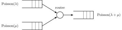
Networking picture: merging. Two independent packet streams feed a router through separate buffers. If the numbers of packets arriving in each buffer during an interval are Poisson(λ) and Poisson(μ), the number of packets in the merged output buffer is Poisson(λ+μ).
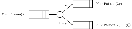
Splitting is the reverse operation: each arriving packet is routed to one of two outputs by an independent coin flip. Given the total count X=n, the number Y sent to the first output is the number of successes in n independent Bernoulli(p) trials. This is a “binomial with a random number of trials.”
Theorem 4.11 (Poisson splitting)
Let X∼Poisson(λ), and suppose that, conditioned on X=n, the random variable Y satisfies
Y∣X=n∼Binomial(n,p).
Let Z=X−Y be the remainder. Then
Y∼Poisson(λp),Z∼Poisson(λ(1−p)),andY⊥Z.
Proof (supplementary).
We compute the joint PMF of (Y,Z) and show that it factors. Fix integers a,b≥0. The event {Y=a,Z=b} is the same as {X=a+b,Y=a} (the total is a+b, of which a went to the first output). By the chain rule,
P(Y=a,Z=b)=P(X=a+b)P(Y=a∣X=a+b)=(a+b)!e−λλa+b⋅(aa+b)pa(1−p)b=(a+b)!e−λλa+b⋅a!b!(a+b)!pa(1−p)b=e−λa!λapa⋅b!λb(1−p)b=Poisson(λp) PMF at aa!e−λp(λp)a⋅Poisson(λ(1−p)) PMF at bb!e−λ(1−p)(λ(1−p))b,(Poisson, then binomial)(expand the binomial coefficient)(cancel (a+b)!, split λa+b)(split e−λ=e−λpe−λ(1−p))
Marginal of Y. Sum over b≥0. The second factor is a PMF in b, so it sums to 1, leaving P(Y=a)=a!e−λp(λp)a. Thus Y∼Poisson(λp). Summing over a instead shows Z∼Poisson(λ(1−p)).
Independence. The joint PMF equals the product of the two marginals for every (a,b), which is the definition of Y⊥Z.
Why the independence is surprising. If the total X were a fixed number n, then Y and Z=n−Y would be perfectly (negatively) dependent: learning Y would tell you Z exactly. It is the randomness of the total count that makes the two outputs independent. A large value of Y suggests X was large, which exactly offsets what it would otherwise say about Z. This is special to the Poisson.
Conditional PMFs and Conditional Expectation
Definition 4.4 (Conditional PMF)
Let X,Y be discrete random variables and let y satisfy pY(y)>0. The conditional PMF of X given Y=y is
pX∣Y(x∣y)≜P(X=x∣Y=y)=pY(y)pX,Y(x,y).
It is a genuine PMF in x. For each fixed y with pY(y)>0:
pX∣Y(x∣y)≥0, since it is a ratio of a probability and a positive number;
it sums to one over x, by marginalizing the joint PMF:
x∑pX∣Y(x∣y)=pY(y)1x∑pX,Y(x,y)=pY(y)pY(y)=1.
So for each fixed value y, “X given Y=y” is just another random variable with its own distribution, and we can take its expectation. (Note that the fraction is pX,Y(x,y)/pY(y), a ratio of PMF values, rather than P(X∩Y)/P(Y), since X and Y are random variables rather than events.)
Definition 4.5 (Conditional expectation given Y=y)
For y with pY(y)>0, the conditional expectation of X given Y=y is
E[X∣Y=y]≜x∑x⋅pX∣Y(x∣y)=x∑x⋅P(X=x∣Y=y).(4.74)
Like any expectation, E[X∣Y=y] is just a real number.
By “sweeping” through the values of y in (4.74), we get a (possibly different) number E[X∣Y=y] for every value y. That is, y↦E[X∣Y=y] is a function of y.
Definition 4.6 (Conditional expectation as a random variable)
Define g(y)=E[X∣Y=y]. The conditional expectation of X given Y is the random variable
E[X∣Y]≜g(Y).
It is a function of Y, and therefore E[X∣Y] is itself a random variable: it takes the value g(y) with probability pY(y).
Notation: E[X∣Y=y] versus E[X∣Y]. These are different objects. E[X∣Y=y] (lowercase y, a specific value) is a number. E[X∣Y] (capital Y) is a random variable.
Example 4.3 (Die roll, conditioned on parity)
Roll a fair six-sided die. Let X be the result and Y=1{X is even}.
Given Y=1, X is uniform on {2,4,6}, so E[X∣Y=1]=32+4+6=4. Given Y=0, X is uniform on {1,3,5}, so E[X∣Y=0]=31+3+5=3. Hence
E[X∣Y]=g(Y)={43if Y=1,if Y=0,i.e.E[X∣Y]=3+Y.
This is a random variable taking the values 3 and 4, each with probability 21. Notice that its mean is 21(3)+21(4)=3.5=E[X]. That is no coincidence, as the next lecture will show.
Law of Iterated Expectation (Tower Rule): TBD next lecture. This was on today’s agenda but was not reached in lecture. It states that E[E[X∣Y]]=E[X]; the total expectation theorem of Section 4.5 is a special case.