Lecture 10: Laws of Large Numbers and the Central Limit Theorem
EECS 126 (UC Berkeley) · Spring 2026 · February 19, 2026
Reading: Bertsekas & Tsitsiklis, Ch. 5; supplementary notes on convergence.
These are my personal notes from Professor Kannan Ramchandran’s EECS 126 (Probability and Random Processes) course at UC Berkeley.
Topics: the weak law of large numbers (WLLN), convergence in probability, almost sure convergence and the strong law of large numbers (SLLN), and the central limit theorem (CLT).
Recap: Concentration Inequalities
The following bounds were derived in Lecture 9; we restate the ones used below.
Theorem 10.1 (Markov’s inequality)
If X≥0 and a>0, then
P(X≥a)≤aE[X].
Theorem 10.2 (Chebyshev’s inequality)
If X has mean μ and variance σ2, then for every c>0,
P(∣X−μ∣≥c)≤c2Var(X)=c2σ2.(10.2)
With c=kσ:
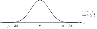
P(∣X−μ∣≥kσ)≤k21.
The left side is the probability that X deviates from its mean by at least c. For k=3, the two tails beyond μ±3σ have total probability at most 91, for any distribution with finite variance.
Theorem 10.3 (Chernoff bound)
For every b,
P(X≥b)≤s>0mine−sbMX(s),MX(s)=E[esX].
Example 10.1 (Chernoff bound for a Gaussian tail)
Let X∼N(0,σ2), so MX(s)=eσ2s2/2 (Lecture 8). With b=kσ,
Formally, for all ε,δ>0 there exists n(ε,δ) such that
P(∣Mn−μ∣≥ε)≤δfor all n≥n(ε,δ).
From (10.12), nε2σ2≤δ⟺n≥ε2δσ2, so n(ε,δ)=ε2δσ2 samples suffice. For example, with σ2=1, ε=0.1, δ=0.05: n≥(0.01)(0.05)1=2000.
What are ε and δ capturing? I had a question of what ε captures in this statement.
ε is the accuracy: how close Mn must be to μ.
δ is the confidence: the probability of a deviation of at least ε is at most δ. (It bounds a probability, not the deviation itself.)
n(ε,δ) is the number of samples needed for a given accuracy and confidence.
In words: for n≥n(ε,δ), ∣Mn−μ∣<ε with probability at least 1−δ.
Convergence in Probability
Definition 10.1 (Convergence in probability)
A sequence Y1,Y2,…converges in probability to a constant a, written Ynpa, if for every ε>0,
n→∞limP(∣Yn−a∣≥ε)=0.
The WLLN says exactly that Mnpμ.
Example 10.2 (Minimum of uniforms)
Let X1,X2,… be i.i.d. Uniform[0,1] and Yn=min(X1,…,Xn). Does Yn converge in probability, and to what?
As we draw more samples, the smallest one should approach 0. Fix 0<ε<1. Since Yn≥0,
P(∣Yn−0∣≥ε)=P(Yn≥ε)=P(min(X1,…,Xn)≥ε)=P(X1≥ε,X2≥ε,…,Xn≥ε)=i=1∏nP(Xi≥ε)=(1−ε)n⟶0as n→∞,(all must be ≥ε)(independence)
since 0<1−ε<1. (For ε≥1 the probability is 0.) Therefore Ynp0.
Example 10.3 (Discrete-time arrival process)
Time runs in slots n=1,2,3,…, grouped into intervals
Ik={2k,2k+1,…,2k+1−1},k=0,1,2,…,
so I0={1}, I1={2,3}, I2={4,…,7}, I3={8,…,15}, and ∣Ik∣=2k. There is exactly 1 arrival in each interval Ik, at a time chosen uniformly at random within Ik. Let
Yn={10if there is an arrival at time n,otherwise.
Each time in Ik is equally likely to hold the arrival, so
As n→∞, the interval index k containing n also goes to ∞, so
n→∞limP(Yn=1)=k→∞lim2k1=0.
For 0<ε≤1, P(∣Yn−0∣≥ε)=P(Yn=1)→0 (and it is 0 for ε>1), so Ynp0.
Converging, yet arrivals keep coming. Initially I was wondering how Yn can converge to 0 when, no matter which n I pick, infinitely many arrivals still come after it. This is why convergence in probability is a weak notion: it only says that at each fixed large n, an arrival at that particular time is unlikely. It says nothing about a single realization of the whole sequence, which still has Yn=1 once in every interval. This weakness belongs to convergence in probability, not to the WLLN itself.
Almost Sure Convergence and the Strong Law
Each outcome ω of the experiment produces a whole realization: an ordinary sequence of numbers Y1(ω),Y2(ω),….
Definition 10.2 (Almost sure convergence)
Ynconverges almost surely (a.s.) to Y, written Yna.s.Y, if
P({ω:n→∞limYn(ω)=Y(ω)})=1.
That is, the realization converges as an ordinary sequence for every outcome outside an event of probability 0.
Theorem 10.5 (Strong law of large numbers)
Let {Xn}n≥1 be i.i.d. with mean μ. Then
P(n→∞limn1i=1∑nXi=μ)=1,i.e.Mna.s.μ.
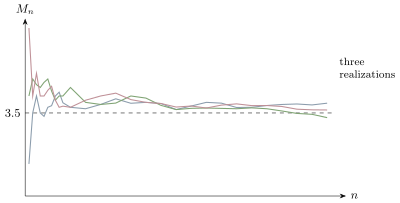
(The proof is beyond the scope of this course.) For fair die rolls, μ=61+2+⋯+6=621=3.5, and every realization of Mn (except on an event of probability 0) converges to 3.5:
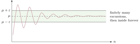
Excursions: SLLN versus WLLN. Initially I was wondering whether the SLLN allows any excursions at all outside a band μ±ε. It does: almost every realization leaves the band only finitely many times, and after some point stays inside forever. Convergence in probability (the WLLN) only requires that, at each fixed large n, few realizations are outside the band; a single realization may still leave it infinitely often.
Theorem 10.6 (Almost sure convergence implies convergence in probability)
If Yna.s.Y, then YnpY. The converse is not necessarily true.
Proof.
Fix ε>0 and let
An=m≥n⋃{∣Ym−Y∣≥ε},
the event that the realization leaves the ε-band at some time m≥n. Then A1⊇A2⊇⋯. An outcome in every An leaves the band infinitely often, so its realization does not converge to Y; hence P(⋂nAn)≤P(Yn→Y)=0. By continuity of probability for decreasing events (a consequence of countable additivity, Lecture 1), P(An)→P(⋂nAn)=0. Since {∣Yn−Y∣≥ε}⊆An,
P(∣Yn−Y∣≥ε)≤P(An)⟶0.
The converse fails: the arrival process. Every realization has exactly one arrival in each interval Ik, so Yn(ω)=1 for infinitely many n and Yn(ω)=0 for infinitely many n. The sequence Yn(ω) never converges, for every outcome ω, so P(Yn→0)=0. Thus Ynp0 but Yn does not converge almost surely.
The Central Limit Theorem
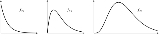
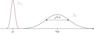
Let X1,X2,… be i.i.d. and Sn=∑i=1nXi. What happens to the distribution of Sn as n grows?
Example 10.4 (Sums of uniforms)
Xi∼Uniform[0,1]. fS1 is a box and fS2 is the triangle from Lecture 8. Convolving once more, fS3(z)=∫z−1zfS2(x)dx:
Standardizing does not make Zn Gaussian. I had a question of whether the CLT just says that Zn becomes Gaussian once it is normalized. E[Zn]=0 and Var(Zn)=1 for every n, but for finite n, Zn is generally not Gaussian (for uniform Xi, Zn even has bounded support). The CLT is a statement about the limit: the CDF of Zn approaches Φ as n→∞.
Definition 10.3 (Convergence in distribution)
Znconverges in distribution to Z, written ZndZ, if
n→∞limP(Zn≤x)=P(Z≤x)
at every x where the CDF of Z is continuous.
Theorem 10.7 (Central limit theorem)
Let X1,X2,… be i.i.d. with mean μ and variance 0<σ2<∞, and Zn=nσSn−nμ. Then for every x∈R,
where Z∼N(0,1) and u is a dummy variable. That is, ZndN(0,1).
Implications.
In the limit, the distribution of Zn “wipes out” all information about the distribution of the Xi except the mean and the variance.
If there are a large number of independent small disturbances, their aggregate effect is approximately normally distributed. This is why the Gaussian is a good model for noise.
The finite-variance assumption is needed: without it, Zn need not approach a Gaussian.
Proof via MGFs.
Assume MX1(s)<∞ for s in an interval around 0. Standardize each term: Yi=σXi−μ, i.i.d. with E[Yi]=0 and E[Yi2]=Var(Yi)=1. Then
Zn=nσSn−nμ=nσ∑i=1n(Xi−μ)=n1i=1∑nYi.
By the MGF properties of Lecture 8 (scaling, then independent sums),
So MZn(s)→es2/2, which is the MGF of N(0,1) (Lecture 8). Finally, we use without proof the continuity theorem: if MZn(s)→MZ(s) for all s in an interval around 0, then ZndZ. Hence ZndN(0,1).
This proof assumes the MGF exists near 0. The CLT holds with only a finite variance; that more general proof uses characteristic functions and is beyond the scope of this course.
![The interval [0, 1] with the part from ε to 1 shaded, labeled P(X_i ≥ ε) = 1 − ε](/courses/eecs126/lecture-10/laws-of-large-numbers-and-the-central-limit-theorem/minimum-of-uniforms.svg)

![The densities of S_1 (a box on [0, 1]), S_2 (a triangle on [0, 2]) and S_3 (a smooth bell-like curve on [0, 3] centered at 1.5)](/courses/eecs126/lecture-10/laws-of-large-numbers-and-the-central-limit-theorem/sums-of-uniforms.svg)