eecs126-full-course-notes.html

EECS 126 Full Course Notes

Lecture 1: Axioms of Probability

EECS 126 (UC Berkeley) · Spring 2026 · January 20, 2026

A probability space provides the mathematical framework for modeling random experiments. In this lecture we define the axioms of probability, introduce sample spaces and events, work through several foundational examples, and derive the birthday paradox bound.

Probability Spaces

Definition 1.1 (Probability space)

A probability space is a triple (Ω,F,P)(\Omega, \FF, \PP) where:

  • Ω\Omega is the sample space: the set of all possible outcomes of the experiment.
  • F⊆2Ω\FF \subseteq 2^{\Omega} is a σ\sigma-algebra of subsets of Ω\Omega, called events.
  • P:F→[0,1]\PP : \FF \to [0,1] is a probability measure satisfying the Kolmogorov axioms.

The elements ω∈Ω\omega \in \Omega are called base outcomes (or samples). A σ\sigma-algebra F\FF is a family of subsets of Ω\Omega that is closed under countable unions, countable intersections, and complements, and that contains Ω\Omega itself. In many discrete settings we simply take F=2Ω\FF = 2^{\Omega} (the power set), so that every subset of Ω\Omega is an event.

Example 1.1 (Tossing two fair coins)

Toss two fair coins. The sample space is

Ω={HH,  HT,  TH,  TT}.\Omega = \{HH,\; HT,\; TH,\; TT\}.

Each base outcome is equally likely, so we assign P({ω})=14\PP(\{\omega\}) = \tfrac{1}{4} for each ω∈Ω\omega \in \Omega. The event space is the power set F=2Ω\FF = 2^{\Omega}, which has ∣F∣=2∣Ω∣=24=16|\FF| = 2^{|\Omega|} = 2^4 = 16 elements.

Example 1.2 (Toss until heads)

Toss a coin repeatedly until the first heads. Then

Ω={H,  TH,  TTH,  TTTH,  …}\Omega = \{H,\; TH,\; TTH,\; TTTH,\; \ldots\}

is a countably infinite sample space.

Example 1.3 (Waiting for a bus)

Wait at a bus stop for the next bus, which arrives at some time in [0,T][0, T]. Now

Ω=[0,T]\Omega = [0, T]

is an uncountably infinite (continuous) sample space. In this setting the choice of F\FF becomes nontrivial; one typically takes F\FF to be the Borel σ\sigma-algebra on [0,T][0,T].

Kolmogorov Axioms

Definition 1.2 (Kolmogorov axioms)

A function P:F→R\PP : \FF \to \RR is a probability measure on (Ω,F)(\Omega, \FF) if it satisfies:

  1. Nonnegativity. P(A)≥0\PP(A) \ge 0 for all A∈FA \in \FF.
  2. Normalization. P(Ω)=1\PP(\Omega) = 1.
  3. Countable additivity. If A1,A2,…∈FA_1, A_2, \ldots \in \FF are pairwise disjoint (Ai∩Aj=∅A_i \cap A_j = \varnothing for i≠ji \ne j), then P ⁣(⋃i≥1Ai)=∑i≥1P(Ai).\PP\!\Bigl(\bigcup_{i \ge 1} A_i\Bigr) = \sum_{i \ge 1} \PP(A_i).

Why countable additivity? In a continuous sample space such as Ω=[0,1]\Omega = [0,1], every individual point has probability zero: P({x})=0\PP(\{x\}) = 0. If we only had finite additivity, we could not recover P([0,1])=1\PP([0,1]) = 1 from the probabilities of individual points. Countable additivity bridges this gap and is essential for the theory of continuous distributions.

Example 1.4 (Biased coin)

Flip a biased coin: heads with probability pp, tails with probability 1−p1 - p. Set

Ω={H,T},F=2Ω={∅,  {H},  {T},  {H,T}}.\Omega = \{H, T\}, \qquad \FF = 2^{\Omega} = \bigl\{\varnothing,\; \{H\},\; \{T\},\; \{H,T\}\bigr\}.

Define

P(H)=p,P(T)=1−p,P(∅)=0,P({H,T})=1.\PP(H) = p, \quad \PP(T) = 1-p, \quad \PP(\varnothing) = 0, \quad \PP(\{H,T\}) = 1.

Then (Ω,F,P)(\Omega, \FF, \PP) is a valid probability space.

Fundamental Probability Facts

The following basic identities are direct consequences of the Kolmogorov axioms.

Theorem 1.1 (Complement rule)

For any event A∈FA \in \FF,

P(Ac)=1−P(A).\PP(A^c) = 1 - \PP(A).
Proof.

Since AA and AcA^c are disjoint with A∪Ac=ΩA \cup A^c = \Omega, countable additivity gives P(A)+P(Ac)=P(Ω)=1\PP(A) + \PP(A^c) = \PP(\Omega) = 1.

Theorem 1.2 (Inclusion–exclusion)

For any two events A,B∈FA, B \in \FF,

P(A∪B)=P(A)+P(B)−P(A∩B).\PP(A \cup B) = \PP(A) + \PP(B) - \PP(A \cap B).

More generally, for events A1,A2,…,AnA_1, A_2, \ldots, A_n,

P ⁣(⋃i=1nAi)=∑iP(Ai)−∑i<jP(Ai∩Aj)+∑i<j<kP(Ai∩Aj∩Ak)−⋯+(−1)n+1 P(A1∩⋯∩An).\begin{aligned} \PP\!\Bigl(\bigcup_{i=1}^{n} A_i\Bigr) = \sum_{i} \PP(A_i) &- \sum_{i < j} \PP(A_i \cap A_j) + \sum_{i < j < k} \PP(A_i \cap A_j \cap A_k) \\ &- \cdots + (-1)^{n+1}\, \PP(A_1 \cap \cdots \cap A_n). \end{aligned}
Theorem 1.3 (Union bound)

For any events A1,…,AnA_1, \ldots, A_n,

P ⁣(⋃i=1nAi)  ≤  ∑i=1nP(Ai).\PP\!\Bigl(\bigcup_{i=1}^{n} A_i\Bigr) \;\le\; \sum_{i=1}^{n} \PP(A_i).
Proof.

Define B1=A1B_1 = A_1 and Bk=Ak∖⋃i<kAiB_k = A_k \setminus \bigcup_{i<k} A_i for k≥2k \ge 2. The BkB_k are disjoint with ⋃Bk=⋃Ak\bigcup B_k = \bigcup A_k, and P(Bk)≤P(Ak)\PP(B_k) \le \PP(A_k), so P(⋃Ak)=∑P(Bk)≤∑P(Ak)\PP(\bigcup A_k) = \sum \PP(B_k) \le \sum \PP(A_k).

Discrete Probability and Counting

In a discrete sample space, the probability of an event is just the sum of the probabilities of its base outcomes:

P(A)=∑ω∈AP({ω}).\PP(A) = \sum_{\omega \in A} \PP(\{\omega\}).
Definition 1.3 (Uniform sample space)

When all outcomes are equally likely, we say Ω\Omega is a uniform sample space, and for any event AA,

P(A)=∣A∣∣Ω∣.\PP(A) = \frac{|A|}{|\Omega|}.

The Birthday Paradox

Example 1.5 (Birthday paradox)

Let nn people be in a room. What is the probability that at least two share a birthday? Let K=365K = 365 and assume birthdays are uniform. Let AA = “at least two people share a birthday.” Compute via the complement:

P(Ac)=K(K−1)(K−2)⋯(K−n+1)Kn=∏j=0n−1(1−jK).\PP(A^c) = \frac{K(K-1)(K-2)\cdots(K-n+1)}{K^n} = \prod_{j=0}^{n-1}\Bigl(1 - \frac{j}{K}\Bigr).

Using 1−x≤e−x1 - x \le e^{-x}:

P(Ac)≤∏j=0n−1e−j/K=e−∑j=0n−1j/K=e−n(n−1)/(2K).\PP(A^c) \le \prod_{j=0}^{n-1} e^{-j/K} = e^{-\sum_{j=0}^{n-1} j/K} = e^{-n(n-1)/(2K)}.
Theorem 1.4 (Birthday bound)

P(A)≥1−e−n(n−1)/(2K)\PP(A) \ge 1 - e^{-n(n-1)/(2K)}. For K=365K = 365 and n=23n = 23, this gives P(A)≥50%\PP(A) \ge 50\%.

Balls-and-bins interpretation. The birthday problem is equivalent to throwing nn balls uniformly into KK bins and asking for the probability of a collision. This connection arises frequently in hashing, load balancing, and networking.

Lecture 2: Conditional Probability and Independence

EECS 126 (UC Berkeley) · Spring 2026 · January 22, 2026

In this lecture we introduce conditional probability, derive the multiplication (chain) rule, state the law of total probability and Bayes’ rule, work through the classic false-positive medical testing example, and then develop the theory of independence and conditional independence.

Conditional Probability

Definition 2.1 (Conditional probability)

Let A,BA, B be events with P(B)>0\PP(B) > 0. The conditional probability of AA given BB is

P(A∣B)=P(A∩B)P(B).\PP(A \mid B) = \frac{\PP(A \cap B)}{\PP(B)}.

Intuitively, P(A∣B)\PP(A \mid B) is the probability that AA occurs when we know that BB has occurred. Conditioning on BB restricts the sample space from Ω\Omega to BB; the event BB becomes the new “Ω\Omega” for AA.

In a uniform sample space, P(A)=∣A∣/∣Ω∣\PP(A) = |A|/|\Omega|. Conditioning on BB gives P(A∣B)=∣A∩B∣/∣B∣\PP(A \mid B) = |A \cap B|/|B|, which is simply the fraction of outcomes in BB that also lie in AA.

Example 2.1 (Two dice – conditioning on the sum)

Roll two standard dice. Let A={1st die is 6}A = \{\text{1st die is 6}\}, B={sum of two dice is 7}B = \{\text{sum of two dice is 7}\}, and C={sum of two dice is 11}C = \{\text{sum of two dice is 11}\}.

Computing P(A∣B)\PP(A \mid B): The outcomes in BB (sum = 7) are {(1,6),(2,5),(3,4),(4,3),(5,2),(6,1)}\{(1,6),(2,5),(3,4),(4,3),(5,2),(6,1)\}, so P(B)=6/36\PP(B) = 6/36. The only outcome in A∩BA \cap B is (6,1)(6,1), so P(A∩B)=1/36\PP(A \cap B) = 1/36. Therefore

P(A∣B)=1/366/36=16.\PP(A \mid B) = \frac{1/36}{6/36} = \frac{1}{6}.

Computing P(A∣C)\PP(A \mid C): The outcomes in CC (sum = 11) are {(5,6),(6,5)}\{(5,6),(6,5)\}, so P(C)=2/36\PP(C) = 2/36. The only outcome in A∩CA \cap C is (6,5)(6,5), so

P(A∣C)=1/362/36=12.\PP(A \mid C) = \frac{1/36}{2/36} = \frac{1}{2}.

Multiplication Rule (Chain Rule)

Theorem 2.1 (Chain rule of probability)

For any events A1,A2,…,AnA_1, A_2, \ldots, A_n with P(A1∩A2∩⋯∩An−1)>0\PP(A_1 \cap A_2 \cap \cdots \cap A_{n-1}) > 0,

P(A1∩A2∩⋯∩An)=P(A1) P(A2∣A1) P(A3∣A1∩A2)⋯P(An∣A1∩⋯∩An−1).\PP(A_1 \cap A_2 \cap \cdots \cap A_n) = \PP(A_1)\,\PP(A_2 \mid A_1)\,\PP(A_3 \mid A_1 \cap A_2) \cdots \PP(A_n \mid A_1 \cap \cdots \cap A_{n-1}).
Proof.

By repeated application of the definition of conditional probability. Write P(A1∩A2)=P(A1) P(A2∣A1)\PP(A_1 \cap A_2) = \PP(A_1)\,\PP(A_2 \mid A_1), then P(A1∩A2∩A3)=P(A1∩A2) P(A3∣A1∩A2)\PP(A_1 \cap A_2 \cap A_3) = \PP(A_1 \cap A_2)\,\PP(A_3 \mid A_1 \cap A_2), and continue inductively. Each factor is well-defined because P(A1∩⋯∩Ak−1)>0\PP(A_1 \cap \cdots \cap A_{k-1}) > 0 implies P(A1∩⋯∩Ak)≤P(A1∩⋯∩Ak−1)\PP(A_1 \cap \cdots \cap A_k) \le \PP(A_1 \cap \cdots \cap A_{k-1}), and we are given the intersection has positive probability up to n−1n-1 terms.

Birthday paradox via the chain rule. The chain rule gives an alternative derivation of the birthday bound. Let Ai={person i doesn’t share a birthday with persons 1,…,i−1}A_i = \{\text{person } i \text{ doesn't share a birthday with persons } 1, \ldots, i-1\}. Then

P(A1∩⋯∩An)=1⋅K−1K⋅K−2K⋯K−(n−1)K=∏j=0n−1(1−jK)≈e−n(n−1)/(2K),\PP(A_1 \cap \cdots \cap A_n) = 1 \cdot \frac{K-1}{K} \cdot \frac{K-2}{K} \cdots \frac{K-(n-1)}{K} = \prod_{j=0}^{n-1}\Bigl(1 - \frac{j}{K}\Bigr) \approx e^{-n(n-1)/(2K)},

recovering the same bound from Lecture 1.

Law of Total Probability

Theorem 2.2 (Law of total probability)

Let A1,A2,…,ANA_1, A_2, \ldots, A_N be a partition of Ω\Omega (i.e. the AiA_i are pairwise disjoint — mutually exclusive — and their union is Ω\Omega — collectively exhaustive). Then for any event BB,

P(B)=∑i=1NP(Ai) P(B∣Ai).\PP(B) = \sum_{i=1}^{N} \PP(A_i)\,\PP(B \mid A_i).
Proof.

Since {Ai}\{A_i\} partitions Ω\Omega, we can decompose BB as B=⋃i=1N(Ai∩B)B = \bigcup_{i=1}^N (A_i \cap B), and these pieces are disjoint. By countable additivity, P(B)=∑i=1NP(Ai∩B)=∑i=1NP(Ai) P(B∣Ai)\PP(B) = \sum_{i=1}^N \PP(A_i \cap B) = \sum_{i=1}^N \PP(A_i)\,\PP(B \mid A_i), where the last step uses the definition of conditional probability.

Bayes’ Rule

Theorem 2.3 (Bayes’ rule)

Let A1,…,ANA_1, \ldots, A_N partition Ω\Omega. Given an event BB with P(B)>0\PP(B) > 0,

P(Ai∣B)=P(B∣Ai) P(Ai)∑j=1NP(B∣Aj) P(Aj).\PP(A_i \mid B) = \frac{\PP(B \mid A_i)\,\PP(A_i)}{\sum_{j=1}^{N} \PP(B \mid A_j)\,\PP(A_j)}.

The numerator uses the definition of conditional probability, and the denominator is P(B)\PP(B) expanded by the law of total probability.

Example 2.2 (False positive quiz – testing for a rare disease)

A medical test for a rare disease has the following properties:

  • If a person has the disease, the test is positive with probability 0.950.95 (sensitivity).
  • If a person does not have the disease, the test is negative with probability 0.950.95 (specificity), i.e. false positive rate =0.05= 0.05.
  • The prior prevalence is P(A)=0.001\PP(A) = 0.001 (1 in 1000 people have the disease).

A person tests positive. What is P(disease∣positive)\PP(\text{disease} \mid \text{positive})?

Define A={has disease}A = \{\text{has disease}\}, B={tests positive}B = \{\text{tests positive}\}. By Bayes’ rule:

P(A∣B)=P(B∣A) P(A)P(B∣A) P(A)+P(B∣Ac) P(Ac)=(0.95)(0.001)(0.95)(0.001)+(0.05)(0.999)≈0.0187.\PP(A \mid B) = \frac{\PP(B \mid A)\,\PP(A)}{\PP(B \mid A)\,\PP(A) + \PP(B \mid A^c)\,\PP(A^c)} = \frac{(0.95)(0.001)}{(0.95)(0.001) + (0.05)(0.999)} \approx 0.0187.

Despite the test being 95% accurate, a positive result only indicates a ≈1.87%\approx 1.87\% chance of actually having the disease. This is because the disease is so rare that the false positives from healthy people vastly outnumber the true positives.

Sensitivity to the prior. If the prior were P(A)=0.01\PP(A) = 0.01 instead (10×10\times more common), then P(A∣B)≈16%\PP(A \mid B) \approx 16\% — still low, but dramatically higher. The base rate (prior) has an enormous effect on the posterior.

Independence

Definition 2.2 (Independence of two events)

Two events AA and BB are independent if the occurrence of one provides no information about the occurrence of the other. Formally:

P(A∣B)=P(A),or equivalently,P(A∩B)=P(A) P(B).\PP(A \mid B) = \PP(A), \qquad \text{or equivalently,} \qquad \PP(A \cap B) = \PP(A)\,\PP(B).

The second form says the joint probability equals the product of the marginals.

Key remarks on independence:

  1. Disjoint ≠\ne independent. A,BA, B disjoint means P(A∩B)=0\PP(A \cap B) = 0. For this to equal P(A)P(B)\PP(A)\PP(B), we need P(A)=0\PP(A) = 0 or P(B)=0\PP(B) = 0. So disjoint events with positive probability are dependent, not independent.
  2. Base outcomes are always dependent. Individual outcomes {ω}\{\omega\} in any finite Ω\Omega are always dependent (knowing one occurred rules out the others).
Example 2.3 (Dice: independence depends on the conditioning event)

Roll two fair dice. Let A={1st die is 6}A = \{\text{1st die is 6}\}, B={sum is 7}B = \{\text{sum is 7}\}, C={sum is 11}C = \{\text{sum is 11}\}.

Are AA and BB independent? P(A∣B)=1/6=P(A)\PP(A \mid B) = 1/6 = \PP(A), so yes, A⊥BA \perp B.

Are AA and CC independent? P(A∣C)=1/2≠1/6=P(A)\PP(A \mid C) = 1/2 \ne 1/6 = \PP(A), so no, AA and CC are dependent. Intuitively, knowing the sum is 11 makes it more likely that the first die was a 6 (since (6,5)(6,5) is one of only two outcomes).

Conditional Independence

Definition 2.3 (Conditional independence)

Events AA and BB are conditionally independent given CC if

P(A∩B∣C)=P(A∣C) P(B∣C).\PP(A \cap B \mid C) = \PP(A \mid C)\,\PP(B \mid C).

Independence and conditional independence are distinct concepts:

  1. Dependent events can become conditionally independent.
  2. Independent events can become conditionally dependent.
Example 2.4 (Two indistinguishable coins)

You have two coins: one is double-headed, the other is double-tailed. You pick one at random and flip it twice. Let Hi={flip i is heads}H_i = \{\text{flip } i \text{ is heads}\}, i=1,2i=1,2.

Q1: Are H1,H2H_1, H_2 (unconditionally) independent? No. P(H1∣H2)=1≠1/2=P(H1)\PP(H_1 \mid H_2) = 1 \ne 1/2 = \PP(H_1). If the second flip is heads, you certainly picked the double-headed coin, so the first flip is heads with certainty.

Q2: Conditioning on the coin, are they independent? Let A={picked the double-headed coin}A = \{\text{picked the double-headed coin}\}. Then P(H1∩H2∣A)=P(H1∣A) P(H2∣H1∩A)=1⋅1=1\PP(H_1 \cap H_2 \mid A) = \PP(H_1 \mid A)\,\PP(H_2 \mid H_1 \cap A) = 1 \cdot 1 = 1, and P(H1∣A) P(H2∣A)=1⋅1=1\PP(H_1 \mid A)\,\PP(H_2 \mid A) = 1 \cdot 1 = 1. These are equal, so H1⊥H2∣AH_1 \perp H_2 \mid A. Once we know which coin was picked, each flip is determined and independent.

Example 2.5 (Fair coin – independent but conditionally dependent)

Toss a fair coin twice. Let H1={1st toss is H}H_1 = \{\text{1st toss is H}\}, H2={2nd toss is H}H_2 = \{\text{2nd toss is H}\}, and D={1st toss≠2nd toss}D = \{\text{1st toss} \ne \text{2nd toss}\}.

Q1: H1⊥H2H_1 \perp H_2? Yes, by independence of fair coin flips.

Q2: H1⊥H2∣DH_1 \perp H_2 \mid D? No. P(H1∣D) P(H2∣D)=12⋅12=14\PP(H_1 \mid D)\,\PP(H_2 \mid D) = \tfrac{1}{2} \cdot \tfrac{1}{2} = \tfrac{1}{4}. But P(H1∩H2∣D)=0\PP(H_1 \cap H_2 \mid D) = 0, since both flips being heads contradicts DD (the flips must differ). Since 0≠1/40 \ne 1/4, the events are conditionally dependent given DD.

Joint Independence vs. Pairwise Independence

Definition 2.4 (Independence of a collection)

Events {Ai}i∈S\{A_i\}_{i \in S} are jointly (mutually) independent if for every subset T⊆ST \subseteq S,

P ⁣(⋂i∈TAi)=∏i∈TP(Ai).\PP\!\Bigl(\bigcap_{i \in T} A_i\Bigr) = \prod_{i \in T} \PP(A_i).

Pairwise independence only requires this for all pairs ∣T∣=2|T| = 2.

Pairwise independence ⇏\nRightarrow joint independence. Consider the fair coin example: H1,H2,DH_1, H_2, D are pairwise independent (check all three pairs), but they are not jointly independent because P(H1∩H2∩D)=0≠P(H1)P(H2)P(D)=1/8\PP(H_1 \cap H_2 \cap D) = 0 \ne \PP(H_1)\PP(H_2)\PP(D) = 1/8.

Renewal: Rolling a 6 Before a 7

Example 2.6 (Roll a sum of 6 before a sum of 7)

Roll two fair dice independently and repeatedly. Let E={a sum of 6 appears before a sum of 7}E = \{\text{a sum of 6 appears before a sum of 7}\}.

The outcomes that sum to 6 are {(1,5),(2,4),(3,3),(4,2),(5,1)}\{(1,5),(2,4),(3,3),(4,2),(5,1)\}, so P(S)=5/36\PP(S) = 5/36 where S={1st roll sums to 6}S = \{\text{1st roll sums to 6}\}. Similarly, P(T)=6/36\PP(T) = 6/36 where T={1st roll sums to 7}T = \{\text{1st roll sums to 7}\}.

By the law of total probability, conditioning on the first roll:

P(E)=P(E∣S) P(S)+P(E∣T) P(T)+P(E∣(S∪T)c) P((S∪T)c).\PP(E) = \PP(E \mid S)\,\PP(S) + \PP(E \mid T)\,\PP(T) + \PP(E \mid (S \cup T)^c)\,\PP((S \cup T)^c).

We have P(E∣S)=1\PP(E \mid S) = 1, P(E∣T)=0\PP(E \mid T) = 0, and P(E∣(S∪T)c)=P(E)\PP(E \mid (S \cup T)^c) = \PP(E) by the renewal/memoryless property (each roll is independent, so if neither 6 nor 7 appears, we restart). Thus

P(E)=1⋅536+0⋅636+P(E)⋅2536.\PP(E) = 1 \cdot \frac{5}{36} + 0 \cdot \frac{6}{36} + \PP(E) \cdot \frac{25}{36}.

Solving: P(E)(1−25/36)=5/36\PP(E)(1 - 25/36) = 5/36, so P(E)(11/36)=5/36\PP(E)(11/36) = 5/36, giving

P(E)=511.\PP(E) = \frac{5}{11}.

Lecture 3: Discrete Random Variables and Expectation

EECS 126 (UC Berkeley) · Spring 2026 · January 27, 2026

We transition from events to random variables — functions that assign numerical values to outcomes — and develop the key tools of expectation, linearity, LOTUS, and variance.

Random Variables and PMFs

Definition 3.1 (Random variable)

A (discrete) random variable is a function X:Ω→RX : \Omega \to \RR that assigns a real number to each outcome ω∈Ω\omega \in \Omega. We write P(X=x)\PP(X = x) for the probability of the event {ω∈Ω:X(ω)=x}\{\omega \in \Omega : X(\omega) = x\}.

Definition 3.2 (Probability mass function)

The probability mass function (PMF) of a discrete random variable XX is the function pX:R→[0,1]p_X : \RR \to [0,1] defined by

pX(x)=P(X=x).p_X(x) = \PP(X = x).

The PMF satisfies ∑x∈XpX(x)=1\sum_{x \in \mathcal{X}} p_X(x) = 1, where X\mathcal{X} denotes the set of all values taken by XX (the support).

Example 3.1 (Functions of random variables)

Let XX be a random variable with pX(x)=1/5p_X(x) = 1/5 for x∈{−2,−1,0,1,2}x \in \{-2, -1, 0, 1, 2\}. Define Y=∣X∣Y = |X|. Then YY takes values in {0,1,2}\{0, 1, 2\} and

pY(y)=∑{x : ∣x∣=y}pX(x)={1/5if y=0,2/5if y=1,2/5if y=2.p_Y(y) = \sum_{\{x\,:\, |x| = y\}} p_X(x) = \begin{cases} 1/5 & \text{if } y = 0, \\ 2/5 & \text{if } y = 1, \\ 2/5 & \text{if } y = 2. \end{cases}

In general, if Y=g(X)Y = g(X), then pY(y)=∑{x:g(x)=y}pX(x)p_Y(y) = \sum_{\{x : g(x) = y\}} p_X(x).

Definition 3.3 (Bernoulli distribution)

X∼Bernoulli⁡(p)X \sim \Bern(p): a single coin toss.

P(X=k)={1−pk=0,pk=1.\PP(X = k) = \begin{cases} 1-p & k = 0, \\ p & k = 1. \end{cases}
Definition 3.4 (Binomial distribution)

X∼Binomial⁡(n,p)X \sim \Bin(n, p): number of successes in nn independent Bernoulli(p)(p) trials.

P(X=k)=(nk)pk(1−p)n−k,k=0,1,…,n.\PP(X = k) = \binom{n}{k} p^k (1-p)^{n-k}, \qquad k = 0, 1, \ldots, n.

Note: ∑k=0n(nk)pk(1−p)n−k=(p+(1−p))n=1\sum_{k=0}^n \binom{n}{k} p^k(1-p)^{n-k} = (p + (1-p))^n = 1 by the binomial theorem, confirming this is a valid PMF.

Definition 3.5 (Geometric distribution)

X∼Geometric⁡(p)X \sim \Geom(p): number of trials until the first success.

P(X=k)=(1−p)k−1p,k=1,2,3,…\PP(X = k) = (1-p)^{k-1} p, \qquad k = 1, 2, 3, \ldots

The geometric distribution is the discrete analog of “waiting time.”

Definition 3.6 (Poisson distribution)

X∼Poisson⁡(λ)X \sim \Pois(\lambda): models the number of arrivals in a fixed interval.

P(X=k)=λke−λk!,k=0,1,2,…\PP(X = k) = \frac{\lambda^k e^{-\lambda}}{k!}, \qquad k = 0, 1, 2, \ldots

The Poisson is the limiting distribution of Binomial⁡(n,λ/n)\Bin(n, \lambda/n) as n→∞n \to \infty, and arises naturally in modeling rare events and arrival processes.

Example 3.2 (Chess match – a PMF computation)*

Alice and Bob play a match: the first to win a game wins the match. If there are 10 consecutive draws, the match is declared drawn. Each game independently: P(A wins)=0.3\PP(\text{A wins}) = 0.3, P(B wins)=0.4\PP(\text{B wins}) = 0.4, P(draw)=0.3\PP(\text{draw}) = 0.3.

Let LL be the duration (number of games). Then for ℓ=1,2,…,9\ell = 1, 2, \ldots, 9:

pL(ℓ)=(0.3)ℓ−1(1−0.3)=(0.3)ℓ−1(0.7),p_L(\ell) = (0.3)^{\ell - 1}(1 - 0.3) = (0.3)^{\ell-1}(0.7),

since the first ℓ−1\ell - 1 games must be draws and the ℓ\ell-th decisive. For ℓ=10\ell = 10: pL(10)=(0.3)9p_L(10) = (0.3)^9 (all 9 games drawn, match ends).

P(Alice wins match)=∑ℓ=19(0.3)ℓ−1(0.3)=0.3∑k=08(0.3)k\PP(\text{Alice wins match}) = \sum_{\ell=1}^{9}(0.3)^{\ell-1}(0.3) = 0.3 \sum_{k=0}^{8}(0.3)^k. Using ∑k=0∞rk=1/(1−r)\sum_{k=0}^{\infty} r^k = 1/(1-r) for ∣r∣<1|r|<1, in the limit of no cap on draws: P(Alice wins)=0.3/(1−0.3)=3/7\PP(\text{Alice wins}) = 0.3/(1-0.3) = 3/7.

Expectation

Definition 3.7 (Expected value)

The expected value (or mean) of a discrete random variable XX is

E[X]=∑ω∈ΩX(ω) P({ω})=∑x∈Xx⋅P(X=x),\EE[X] = \sum_{\omega \in \Omega} X(\omega)\,\PP(\{\omega\}) = \sum_{x \in \mathcal{X}} x \cdot \PP(X = x),

provided the sum converges absolutely (i.e. ∑∣x∣ P(X=x)<∞\sum |x|\,\PP(X=x) < \infty).

Theorem 3.1 (Linearity of expectation)

For any random variables X,YX, Y (not necessarily independent) and constant cc:

E[X+Y]=E[X]+E[Y],E[cX]=c E[X].\EE[X + Y] = \EE[X] + \EE[Y], \qquad \EE[cX] = c\,\EE[X].

No independence assumption is needed. This is the single most useful property of expectation.

Definition 3.8 (Indicator random variable)

For an event AA, the indicator 1A\mathbf{1}_A is

1A(ω)={1ω∈A,0ω∉A.\mathbf{1}_A(\omega) = \begin{cases} 1 & \omega \in A, \\ 0 & \omega \notin A. \end{cases}

Observe that 1A∼Bernoulli⁡(P(A))\mathbf{1}_A \sim \Bern(\PP(A)), so E[1A]=P(A)\EE[\mathbf{1}_A] = \PP(A).

Example 3.3 (Seats on a plane)

A full flight has nn passengers with assigned seats, but every passenger ignores their assignment and sits in a uniformly random seat. What is E[number who sit in their own seat]\EE[\text{number who sit in their own seat}]?

Let Xi=1{passenger i sits in their own seat}X_i = \mathbf{1}\{\text{passenger } i \text{ sits in their own seat}\}. Then X=X1+X2+⋯+XnX = X_1 + X_2 + \cdots + X_n. The XiX_i are not independent (if n=2n = 2 and passenger 1 is in their seat, passenger 2 must be too). But linearity of expectation does not require independence:

E[X]=∑i=1nE[Xi]=∑i=1nP(passenger i is in their seat)=n⋅1n=1.\EE[X] = \sum_{i=1}^n \EE[X_i] = \sum_{i=1}^n \PP(\text{passenger } i \text{ is in their seat}) = n \cdot \frac{1}{n} = 1.

Regardless of the number of passengers, on average exactly 1 person sits in their own seat.

LOTUS (Law of the Unconscious Statistician)

Theorem 3.2 (LOTUS)

If XX is a discrete random variable and g:R→Rg : \RR \to \RR is any function, then

E[g(X)]=∑x∈Xg(x) P(X=x).\EE[g(X)] = \sum_{x \in \mathcal{X}} g(x)\,\PP(X = x).

More generally, for a function of several random variables:

E[f(X1,…,Xn)]=∑x1,…,xnf(x1,…,xn) pX1,…,Xn(x1,…,xn).\EE[f(X_1, \ldots, X_n)] = \sum_{x_1, \ldots, x_n} f(x_1, \ldots, x_n)\, p_{X_1, \ldots, X_n}(x_1, \ldots, x_n).

The name reflects that one can compute E[g(X)]\EE[g(X)] directly from the distribution of XX, without first finding the distribution of Y=g(X)Y = g(X).

Independence of Random Variables

Definition 3.9 (Independent random variables)

Random variables XX and YY are independent (written X⊥YX \perp Y) if their joint distribution factors into the product of the marginals:

P(X=x, Y=y)=P(X=x) P(Y=y)for all x,y.\PP(X = x,\, Y = y) = \PP(X = x)\,\PP(Y = y) \quad \text{for all } x, y.
Theorem 3.3 (Expectation of a product of independent RVs)

If X⊥YX \perp Y, then

E[XY]=E[X] E[Y].\EE[XY] = \EE[X]\,\EE[Y].
Proof.

By LOTUS and independence:

E[XY]=∑x,yxy pX,Y(x,y)=∑x,yxy pX(x) pY(y)=(∑xx pX(x))(∑yy pY(y))=E[X] E[Y].\begin{aligned} \EE[XY] &= \sum_{x,y} xy\, p_{X,Y}(x,y) = \sum_{x,y} xy\, p_X(x)\, p_Y(y) \\ &= \Bigl(\sum_x x\, p_X(x)\Bigr)\Bigl(\sum_y y\, p_Y(y)\Bigr) = \EE[X]\,\EE[Y]. \end{aligned}

The key step is factoring the joint PMF into marginals (by independence), which allows separating the double sum into a product of single sums.

The converse is false. E[XY]=E[X]E[Y]\EE[XY] = \EE[X]\EE[Y] does not imply X⊥YX \perp Y. The condition E[XY]=E[X]E[Y]\EE[XY] = \EE[X]\EE[Y] is called uncorrelation, which is strictly weaker than independence. As an exercise, construct dependent random variables that are uncorrelated.

Tail Sum Formula

Theorem 3.4 (Tail sum formula)

Let XX be a random variable taking values in N={0,1,2,…}\NN = \{0, 1, 2, \ldots\}. Then

E[X]=∑k=1∞P(X≥k).\EE[X] = \sum_{k=1}^{\infty} \PP(X \ge k).
Proof.

Starting from the definition of expectation:

E[X]=∑k=1∞k P(X=k)=∑k=1∞∑j=1k1⋅P(X=k)=∑j=1∞∑k=j∞P(X=k)=∑j=1∞P(X≥j).\begin{aligned} \EE[X] &= \sum_{k=1}^{\infty} k\,\PP(X = k) = \sum_{k=1}^{\infty} \sum_{j=1}^{k} 1 \cdot \PP(X = k) \\ &= \sum_{j=1}^{\infty} \sum_{k=j}^{\infty} \PP(X = k) = \sum_{j=1}^{\infty} \PP(X \ge j). \end{aligned}

The key step is writing k=∑j=1k1k = \sum_{j=1}^k 1 to introduce a double sum, then swapping the order of summation (Tonelli’s theorem ensures this is valid for nonnegative terms). Geometrically, this corresponds to “counting vertically then horizontally”: instead of weighting each column kk by its height kk, we sum across rows j=1,2,…j = 1, 2, \ldots, each contributing P(X≥j)\PP(X \ge j).

Intuition for the tail sum. Think of E[X]\EE[X] as the total area under the “staircase” of the survival function P(X≥k)\PP(X \ge k). Each unit step at height kk contributes P(X≥k)\PP(X \ge k) to the total. This is the same idea as computing the area under a curve by integrating horizontally rather than vertically.

Variance

Definition 3.10 (Variance and standard deviation)

The variance of XX measures the spread of XX around its mean:

Var⁡(X)≜σX2≜E[(X−E[X])2].\Var(X) \triangleq \sigma_X^2 \triangleq \EE\bigl[(X - \EE[X])^2\bigr].

The standard deviation is σX=Var⁡(X)\sigma_X = \sqrt{\Var(X)}.

An equivalent computational formula (often easier to use):

Var⁡(X)=E[X2]−(E[X])2.\Var(X) = \EE[X^2] - (\EE[X])^2.
Derivation of the computational formula.

Expand the square using linearity:

Var⁡(X)=E[(X−E[X])2]=E[X2−2X E[X]+(E[X])2]=E[X2]−2 E[X] E[X]+(E[X])2=E[X2]−(E[X])2.\begin{aligned} \Var(X) &= \EE[(X - \EE[X])^2] = \EE[X^2 - 2X\,\EE[X] + (\EE[X])^2] \\ &= \EE[X^2] - 2\,\EE[X]\,\EE[X] + (\EE[X])^2 = \EE[X^2] - (\EE[X])^2. \end{aligned}

Note that E[X]\EE[X] is a constant, so E[2X⋅E[X]]=2 E[X]⋅E[X]\EE[2X \cdot \EE[X]] = 2\,\EE[X] \cdot \EE[X] and E[(E[X])2]=(E[X])2\EE[(\EE[X])^2] = (\EE[X])^2.

Theorem 3.5 (Scaling property of variance)

For constants a,c∈Ra, c \in \RR:

Var⁡(aX+c)=a2 Var⁡(X).\Var(aX + c) = a^2\,\Var(X).

Adding a constant shifts the mean but does not change the spread. Scaling by aa scales the variance by a2a^2 (and the standard deviation by ∣a∣|a|).

Proof.

Let μ=E[X]\mu = \EE[X]. Then E[aX+c]=aμ+c\EE[aX + c] = a\mu + c, so

Var⁡(aX+c)=E[(aX+c−aμ−c)2]=E[(a(X−μ))2]=a2 E[(X−μ)2]=a2 Var⁡(X).\Var(aX + c) = \EE[(aX + c - a\mu - c)^2] = \EE[(a(X - \mu))^2] = a^2\,\EE[(X - \mu)^2] = a^2\,\Var(X).

Coming up next lecture: covariance Cov⁡(X,Y)\Cov(X, Y), variance of sums, and the beginning of continuous random variables.

Lecture 4: Variance, Covariance, and Common Discrete Distributions

EECS 126 (UC Berkeley) · Spring 2026 · January 29, 2026

Reading: Bertsekas & Tsitsiklis, Ch. 2; §4.2–4.3. Ch. 3 next week.

These are my personal notes from Professor Kannan Ramchandran’s EECS 126 (Probability and Random Processes) course at UC Berkeley.

Last lecture we defined expectation and variance for a single random variable. In this lecture we study how variance behaves for sums of random variables, which leads to covariance and the correlation coefficient. We then compute the mean and variance of the four workhorse discrete distributions (Bernoulli, binomial, geometric, Poisson), apply these to the coupon collector problem, prove the memoryless property of the geometric distribution, study how Poisson random variables merge and split, and finally introduce conditional expectation.

Variance of Sums and Covariance

Recall from Lecture 3 the two forms of the variance,

Var⁡(X)=E[(X−E[X])2]=E[X2]−(E[X])2,\Var(X) = \EE\bigl[(X - \EE[X])^2\bigr] = \EE[X^2] - (\EE[X])^2,

and the scaling property

Var⁡(aX+c)=a2 Var⁡(X).\Var(aX + c) = a^2\,\Var(X).

Shifts by a constant cc are not recorded in variance calculations: shifting every outcome by cc moves the mean by cc as well, so the deviations X−E[X]X - \EE[X] are unchanged.

The natural next question is: what is the variance of a sum X+YX + Y? Unlike the mean, the answer depends on how XX and YY interact.

Theorem 4.1 (Variance of a sum)

For any random variables X,YX, Y with finite variances,

Var⁡(X+Y)=Var⁡(X)+Var⁡(Y)+2(E[XY]−E[X] E[Y]).(4.3)\Var(X + Y) = \Var(X) + \Var(Y) + 2\bigl(\EE[XY] - \EE[X]\,\EE[Y]\bigr). \tag{4.3}
Proof. Var⁡(X+Y)=E[(X+Y)2]−(E[X+Y])2=E[X2+2XY+Y2]−(E[X]+E[Y])2=E[X2]+2 E[XY]+E[Y2]−(E[X])2−2 E[X] E[Y]−(E[Y])2=E[X2]−(E[X])2⏟Var⁡(X)  +  E[Y2]−(E[Y])2⏟Var⁡(Y)  +  2 E[XY]−2 E[X] E[Y]=Var⁡(X)+Var⁡(Y)+2(E[XY]−E[X] E[Y]).\begin{aligned} \Var(X+Y) &= \EE\bigl[(X+Y)^2\bigr] - \bigl(\EE[X+Y]\bigr)^2 \\ &= \EE\bigl[X^2 + 2XY + Y^2\bigr] - \bigl(\EE[X] + \EE[Y]\bigr)^2 \\ &= \EE[X^2] + 2\,\EE[XY] + \EE[Y^2] - (\EE[X])^2 - 2\,\EE[X]\,\EE[Y] - (\EE[Y])^2 \\ &= \underbrace{\EE[X^2] - (\EE[X])^2}_{\Var(X)} \;+\; \underbrace{\EE[Y^2] - (\EE[Y])^2}_{\Var(Y)} \;+\; 2\,\EE[XY] - 2\,\EE[X]\,\EE[Y] \\ &= \Var(X) + \Var(Y) + 2\bigl(\EE[XY] - \EE[X]\,\EE[Y]\bigr). \end{aligned}

No independence was used. The derivation above holds for any XX and YY. Independence only enters at the very end, where it makes the cross term vanish (Corollary 4.1 below).

The cross term in (4.3) is important enough to get its own name.

Definition 4.1 (Covariance)

The covariance of random variables XX and YY is

Cov⁡(X,Y)≜E[(X−E[X])(Y−E[Y])]=E[XY]−E[X] E[Y].\Cov(X, Y) \triangleq \EE\bigl[(X - \EE[X])(Y - \EE[Y])\bigr] = \EE[XY] - \EE[X]\,\EE[Y].

In particular, Cov⁡(X,X)=Var⁡(X)\Cov(X, X) = \Var(X). With this notation,

Var⁡(X+Y)=Var⁡(X)+Var⁡(Y)+2 Cov⁡(X,Y).\Var(X + Y) = \Var(X) + \Var(Y) + 2\,\Cov(X, Y).
Equivalence of the two forms.

Write μX=E[X]\mu_X = \EE[X] and μY=E[Y]\mu_Y = \EE[Y], which are constants. Expanding the product and using linearity,

E[(X−μX)(Y−μY)]=E[XY−μYX−μXY+μXμY]=E[XY]−μY E[X]−μX E[Y]+μXμY=E[XY]−μYμX−μXμY+μXμY=E[XY]−μXμY.\begin{aligned} \EE\bigl[(X - \mu_X)(Y - \mu_Y)\bigr] &= \EE\bigl[XY - \mu_Y X - \mu_X Y + \mu_X\mu_Y\bigr] \\ &= \EE[XY] - \mu_Y\,\EE[X] - \mu_X\,\EE[Y] + \mu_X\mu_Y \\ &= \EE[XY] - \mu_Y\mu_X - \mu_X\mu_Y + \mu_X\mu_Y \\ &= \EE[XY] - \mu_X\mu_Y. \end{aligned}

Interpreting the sign. Cov⁡(X,Y)>0\Cov(X,Y) > 0 means XX and YY tend to be above their means together (and below their means together). Cov⁡(X,Y)<0\Cov(X,Y) < 0 means when one is above its mean, the other tends to be below. For a sum, positive covariance inflates the spread and negative covariance dampens it.

Corollary 4.1 (Independent summands)

If X⊥YX \perp Y, then Cov⁡(X,Y)=0\Cov(X, Y) = 0, and therefore

Var⁡(X+Y)=Var⁡(X)+Var⁡(Y).\Var(X + Y) = \Var(X) + \Var(Y).
Proof.

In Lecture 3 we proved that X⊥YX \perp Y implies E[XY]=E[X] E[Y]\EE[XY] = \EE[X]\,\EE[Y]. Hence Cov⁡(X,Y)=E[XY]−E[X] E[Y]=0\Cov(X,Y) = \EE[XY] - \EE[X]\,\EE[Y] = 0, and the cross term in (4.3) vanishes.

Corollary 4.2 (Variance of a sum of many random variables)

For random variables X1,…,XnX_1, \ldots, X_n with finite variances,

Var⁡(∑i=1nXi)=∑i=1nVar⁡(Xi)+2∑i<jCov⁡(Xi,Xj).\Var\Bigl(\sum_{i=1}^n X_i\Bigr) = \sum_{i=1}^n \Var(X_i) + 2\sum_{i<j} \Cov(X_i, X_j).

In particular, if the XiX_i are independent (in fact, pairwise uncorrelated is enough), then

Var⁡(∑i=1nXi)=∑i=1nVar⁡(Xi).\Var\Bigl(\sum_{i=1}^n X_i\Bigr) = \sum_{i=1}^n \Var(X_i).
Proof.

Let μi=E[Xi]\mu_i = \EE[X_i]. Since E[∑iXi]=∑iμi\EE[\sum_i X_i] = \sum_i \mu_i, the centered sum is ∑i(Xi−μi)\sum_i (X_i - \mu_i). Squaring a sum gives a double sum over all pairs (i,j)(i, j):

Var⁡(∑iXi)=E[(∑i(Xi−μi))2]=E[∑i∑j(Xi−μi)(Xj−μj)]=∑i∑jCov⁡(Xi,Xj).\begin{aligned} \Var\Bigl(\sum_{i} X_i\Bigr) &= \EE\Bigl[\Bigl(\sum_{i} (X_i - \mu_i)\Bigr)^2\Bigr] = \EE\Bigl[\sum_{i}\sum_{j} (X_i - \mu_i)(X_j - \mu_j)\Bigr] \\ &= \sum_{i}\sum_{j} \Cov(X_i, X_j). \end{aligned}

The diagonal terms i=ji = j give Cov⁡(Xi,Xi)=Var⁡(Xi)\Cov(X_i, X_i) = \Var(X_i). The off-diagonal terms come in symmetric pairs, Cov⁡(Xi,Xj)=Cov⁡(Xj,Xi)\Cov(X_i, X_j) = \Cov(X_j, X_i), so they contribute 2∑i<jCov⁡(Xi,Xj)2\sum_{i<j}\Cov(X_i,X_j). If every pair is uncorrelated, all off-diagonal terms are zero.

Uncorrelated does not imply independent. Covariance only detects linear dependence. For example, let XX be uniform on {−1,0,1}\{-1, 0, 1\} and Y=X2Y = X^2. Then E[X]=0\EE[X] = 0 and E[XY]=E[X3]=13(−1)+13(0)+13(1)=0\EE[XY] = \EE[X^3] = \tfrac13(-1) + \tfrac13(0) + \tfrac13(1) = 0, so Cov⁡(X,Y)=0−0⋅E[Y]=0\Cov(X, Y) = 0 - 0 \cdot \EE[Y] = 0. But YY is completely determined by XX: for instance P(Y=0∣X=0)=1≠13=P(Y=0)\PP(Y = 0 \mid X = 0) = 1 \ne \tfrac13 = \PP(Y = 0). This was a question Ramchandran asked us at end of previous lecture.

The Correlation Coefficient

Covariance has units (units of XX times units of YY), so its size alone does not tell us how strongly two variables are related. Normalizing by the standard deviations removes the units.

Definition 4.2 (Correlation coefficient)

For random variables X,YX, Y with Var⁡(X)>0\Var(X) > 0 and Var⁡(Y)>0\Var(Y) > 0, the correlation coefficient is

ρ(X,Y)≜Cov⁡(X,Y)Var⁡(X) Var⁡(Y).\rho(X, Y) \triangleq \frac{\Cov(X, Y)}{\sqrt{\Var(X)}\,\sqrt{\Var(Y)}}.

Ramchandran’s vector analogy. Think of random variables as vectors, with “dot product” ⟨U,V⟩=E[UV]\langle U, V\rangle = \EE[UV] and “length” E[U2]\sqrt{\EE[U^2]}. For the centered variables U=X−E[X]U = X - \EE[X] and V=Y−E[Y]V = Y - \EE[Y]:

  • the dot product is E[UV]=Cov⁡(X,Y)\EE[UV] = \Cov(X, Y);
  • the lengths are E[U2]=Var⁡(X)\sqrt{\EE[U^2]} = \sqrt{\Var(X)} and E[V2]=Var⁡(Y)\sqrt{\EE[V^2]} = \sqrt{\Var(Y)}.

So ρ\rho plays the role of cos⁡θ=u⋅v∣u∣ ∣v∣\cos\theta = \dfrac{u \cdot v}{|u|\,|v|}, the cosine of the angle between two vectors. For ordinary vectors, the Cauchy–Schwarz inequality ∣u⋅v∣≤∣u∣ ∣v∣|u \cdot v| \le |u|\,|v| forces −1≤cos⁡θ≤1-1 \le \cos\theta \le 1. The same inequality, proved for random variables below, forces −1≤ρ≤1-1 \le \rho \le 1.

Lemma 4.1 (Cauchy–Schwarz inequality for random variables)

For any random variables U,VU, V with E[U2]<∞\EE[U^2] < \infty and E[V2]<∞\EE[V^2] < \infty,

(E[UV])2≤E[U2] E[V2].\bigl(\EE[UV]\bigr)^2 \le \EE[U^2]\,\EE[V^2].
Proof.

Case 1: E[V2]=0\EE[V^2] = 0. Since V2≥0V^2 \ge 0 and its mean is 00, we must have V=0V = 0 with probability 11. Then UV=0UV = 0 with probability 11, so E[UV]=0\EE[UV] = 0 and both sides equal 00.

Case 2: E[V2]>0\EE[V^2] > 0. For every real number tt, the random variable (U−tV)2(U - tV)^2 is nonnegative, so its expectation is nonnegative. Expanding with linearity:

0≤E[(U−tV)2]=E[U2]−2t E[UV]+t2 E[V2].0 \le \EE\bigl[(U - tV)^2\bigr] = \EE[U^2] - 2t\,\EE[UV] + t^2\,\EE[V^2].

This holds for every tt, so choose the tt that minimizes the right-hand side, namely t⋆=E[UV]/E[V2]t^\star = \EE[UV]/\EE[V^2]. Substituting,

0≤E[U2]−2 E[UV]E[V2] E[UV]+(E[UV])2(E[V2])2 E[V2]=E[U2]−2 (E[UV])2E[V2]+(E[UV])2E[V2]=E[U2]−(E[UV])2E[V2].\begin{aligned} 0 &\le \EE[U^2] - 2\,\frac{\EE[UV]}{\EE[V^2]}\,\EE[UV] + \frac{(\EE[UV])^2}{(\EE[V^2])^2}\,\EE[V^2] \\ &= \EE[U^2] - 2\,\frac{(\EE[UV])^2}{\EE[V^2]} + \frac{(\EE[UV])^2}{\EE[V^2]} \\ &= \EE[U^2] - \frac{(\EE[UV])^2}{\EE[V^2]}. \end{aligned}

Multiplying both sides by E[V2]>0\EE[V^2] > 0 gives (E[UV])2≤E[U2] E[V2](\EE[UV])^2 \le \EE[U^2]\,\EE[V^2].

Theorem 4.2 (Range of the correlation coefficient)

Whenever ρ(X,Y)\rho(X, Y) is defined,

−1≤ρ(X,Y)≤1.-1 \le \rho(X, Y) \le 1.
Proof.

Apply Cauchy–Schwarz to the centered variables U=X−E[X]U = X - \EE[X] and V=Y−E[Y]V = Y - \EE[Y]. By definition, E[UV]=Cov⁡(X,Y)\EE[UV] = \Cov(X,Y), E[U2]=Var⁡(X)\EE[U^2] = \Var(X), and E[V2]=Var⁡(Y)\EE[V^2] = \Var(Y), so

(Cov⁡(X,Y))2≤Var⁡(X) Var⁡(Y).\bigl(\Cov(X,Y)\bigr)^2 \le \Var(X)\,\Var(Y).

Taking square roots, ∣Cov⁡(X,Y)∣≤Var⁡(X)Var⁡(Y)|\Cov(X,Y)| \le \sqrt{\Var(X)}\sqrt{\Var(Y)}. Dividing by the (positive) right-hand side gives ∣ρ(X,Y)∣≤1|\rho(X,Y)| \le 1.

Extreme and zero values. ∣ρ∣=1|\rho| = 1 exactly when equality holds in Cauchy–Schwarz, which happens when U−t⋆V=0U - t^\star V = 0 with probability 11, i.e. when YY is an exact linear function Y=aX+bY = aX + b of XX (with ρ=+1\rho = +1 if a>0a > 0 and ρ=−1\rho = -1 if a<0a < 0). At the other end, ρ=0\rho = 0 means uncorrelated, which, as we just saw, is weaker than independent.

Mean and Variance of Common Distributions

We now compute E[X]\EE[X] and Var⁡(X)\Var(X) for the four distributions introduced in Lecture 3. A recurring theme: the direct sums are often messy, and a better representation of the random variable makes the computation easy.

Bernoulli

Theorem 4.3 (Bernoulli mean and variance)

If X∼Bernoulli⁡(p)X \sim \Bern(p), then

E[X]=p,Var⁡(X)=p(1−p).\EE[X] = p, \qquad \Var(X) = p(1-p).
Proof.

XX takes only the values 00 and 11, with P(X=1)=p\PP(X=1) = p and P(X=0)=1−p\PP(X=0) = 1-p.

E[X]=1⋅P(X=1)+0⋅P(X=0)=1⋅p+0=p.\EE[X] = 1 \cdot \PP(X = 1) + 0 \cdot \PP(X = 0) = 1 \cdot p + 0 = p.

For the second moment, by LOTUS,

E[X2]=∑xx2 P(X=x)=12⋅P(X=1)+02⋅P(X=0)=p.\EE[X^2] = \sum_{x} x^2\,\PP(X = x) = 1^2 \cdot \PP(X = 1) + 0^2 \cdot \PP(X = 0) = p.

Therefore

Var⁡(X)=E[X2]−(E[X])2=p−p2=p(1−p).\Var(X) = \EE[X^2] - (\EE[X])^2 = p - p^2 = p(1-p).

Binomial

Theorem 4.4 (Binomial mean and variance)

If X∼Binomial⁡(n,p)X \sim \Bin(n, p), then

E[X]=np,Var⁡(X)=np(1−p).\EE[X] = np, \qquad \Var(X) = np(1-p).

The direct approach is

E[X]=∑x=0nx⋅P(X=x)=∑x=0nx(nx)px(1−p)n−x,\EE[X] = \sum_{x=0}^{n} x \cdot \PP(X = x) = \sum_{x=0}^{n} x \binom{n}{x} p^x (1-p)^{n-x},

which is doable but unpleasant. Instead, think of the binomial as a sum of nn Bernoulli trials.

Proof.

Let Xi=1{trial i is a success}X_i = \mathbf{1}\{\text{trial } i \text{ is a success}\} for i=1,…,ni = 1, \ldots, n. Each Xi∼Bernoulli⁡(p)X_i \sim \Bern(p), the XiX_i are independent (the trials are independent), and the total number of successes is

X=X1+X2+⋯+Xn.X = X_1 + X_2 + \cdots + X_n.

Mean. By linearity of expectation (which needs no independence),

E[X]=∑i=1nE[Xi]=∑i=1np=np.\EE[X] = \sum_{i=1}^{n} \EE[X_i] = \sum_{i=1}^{n} p = np.

Variance. Because the XiX_i are independent, Corollary 4.2 lets us add the variances:

Var⁡(X)=∑i=1nVar⁡(Xi)=∑i=1np(1−p)=np(1−p).\Var(X) = \sum_{i=1}^{n} \Var(X_i) = \sum_{i=1}^{n} p(1-p) = np(1-p).

Applying direct sum gives us the same result: Using the identity x(nx)=n(n−1x−1)x\binom{n}{x} = n\binom{n-1}{x-1} for x≥1x \ge 1 (the x=0x = 0 term is zero),

E[X]=∑x=1nn(n−1x−1)px(1−p)n−x=np∑x=1n(n−1x−1)px−1(1−p)(n−1)−(x−1)=np∑j=0n−1(n−1j)pj(1−p)(n−1)−j=np (p+(1−p))n−1=np,\begin{aligned} \EE[X] &= \sum_{x=1}^{n} n\binom{n-1}{x-1} p^x (1-p)^{n-x} = np \sum_{x=1}^{n} \binom{n-1}{x-1} p^{x-1}(1-p)^{(n-1)-(x-1)} \\ &= np \sum_{j=0}^{n-1} \binom{n-1}{j} p^{j}(1-p)^{(n-1)-j} = np\,\bigl(p + (1-p)\bigr)^{n-1} = np, \end{aligned}

where we substituted j=x−1j = x - 1 and used the binomial theorem. The indicator method reaches the same answer with far less algebra.

Geometric

Recall that X∼Geometric⁡(p)X \sim \Geom(p) counts the number of independent trials up to and including the first success:

pX(k)=P(X=k)=(1−p)k−1 p,k=1,2,3,…p_X(k) = \PP(X = k) = (1-p)^{k-1}\,p, \qquad k = 1, 2, 3, \ldots

Reading the PMF. Here kk marks the trial on which the first Success occurs (k=Sk = S). So pX(k)p_X(k) is the probability that the first success happens on trial kk: the first k−1k - 1 trials are failures (probability (1−p)k−1(1-p)^{k-1}) and trial kk is a success (probability pp). Note that pX(k)p_X(k) is not the probability of kk successes; a geometric random variable always records exactly one success, and kk counts how long we waited for it.

Definition 4.3 (Survival function)

For an integer-valued random variable XX, the survival function (or tail) is k↦P(X>k)k \mapsto \PP(X > k). For X∼Geometric⁡(p)X \sim \Geom(p),

P(X>k)=(1−p)k,k=0,1,2,…(4.27)\PP(X > k) = (1-p)^k, \qquad k = 0, 1, 2, \ldots \tag{4.27}
Proof.

The event {X>k}\{X > k\} means “no success in the first kk trials,” i.e. we tried kk times and failed every time. The trials are independent and each fails with probability 1−p1-p, so P(X>k)=(1−p)⋯(1−p)⏟k times=(1−p)k\PP(X > k) = \underbrace{(1-p)\cdots(1-p)}_{k \text{ times}} = (1-p)^k.

Theorem 4.5 (Geometric mean)

If X∼Geometric⁡(p)X \sim \Geom(p) with 0<p≤10 < p \le 1, then

E[X]=1p.\EE[X] = \frac{1}{p}.

The direct sum E[X]=∑k=1∞k(1−p)k−1p\EE[X] = \sum_{k=1}^\infty k(1-p)^{k-1}p requires a trick. A better method is the tail sum formula from Lecture 3, which applies because XX takes values in the nonnegative integers.

Proof.

By the tail sum formula,

E[X]=∑k=1∞P(X≥k).\EE[X] = \sum_{k=1}^{\infty} \PP(X \ge k).

For integer-valued XX, {X≥k}={X>k−1}\{X \ge k\} = \{X > k - 1\}. Substituting j=k−1j = k - 1 (so jj runs from 00 to ∞\infty),

E[X]=∑k=1∞P(X>k−1)=∑j=0∞P(X>j).\EE[X] = \sum_{k=1}^{\infty} \PP(X > k-1) = \sum_{j=0}^{\infty} \PP(X > j).

Now plug in the survival function (4.27):

E[X]=∑j=0∞(1−p)j.\EE[X] = \sum_{j=0}^{\infty} (1-p)^j.

This is a geometric series ∑j≥0xj\sum_{j \ge 0} x^j with ratio x=1−px = 1 - p. Since 0<p≤10 < p \le 1 we have ∣x∣<1|x| < 1, so the series converges to 1/(1−x)1/(1-x):

E[X]=11−(1−p)=1p.\EE[X] = \frac{1}{1 - (1-p)} = \frac{1}{p}.

Exam note: tail sum formula will be on exam. For a random variable XX taking values in {0,1,2,…}\{0, 1, 2, \ldots\},

E[X]=∑k=1∞P(X≥k)=∑k=0∞P(X>k).\EE[X] = \sum_{k=1}^{\infty} \PP(X \ge k) = \sum_{k=0}^{\infty} \PP(X > k).

It expresses the mean as the sum of the tail probabilities. It follows from writing X=∑k=1∞1{X≥k}X = \sum_{k=1}^{\infty} \mathbf{1}\{X \ge k\} and taking expectations of both sides.

The direct sum, for comparison. Differentiating the geometric series ∑k≥0xk=11−x\sum_{k\ge0} x^k = \frac{1}{1-x} term by term (valid for ∣x∣<1|x|<1) gives ∑k≥1kxk−1=1(1−x)2\sum_{k\ge1} k x^{k-1} = \frac{1}{(1-x)^2}. With x=1−px = 1-p,

E[X]=p∑k=1∞k(1−p)k−1=p⋅1(1−(1−p))2=p⋅1p2=1p.\EE[X] = p\sum_{k=1}^{\infty} k(1-p)^{k-1} = p \cdot \frac{1}{(1-(1-p))^2} = p \cdot \frac{1}{p^2} = \frac{1}{p}.

The variance of the geometric is derived in Section 4.5, using the memoryless property.

Poisson

Theorem 4.6 (Poisson mean and variance)

If X∼Poisson⁡(λ)X \sim \Pois(\lambda), so that pX(k)=e−λλkk!p_X(k) = \dfrac{e^{-\lambda}\lambda^k}{k!} for k=0,1,2,…k = 0, 1, 2, \ldots, then

E[X]=λ,Var⁡(X)=λ.\EE[X] = \lambda, \qquad \Var(X) = \lambda.

Both computations rely on the Taylor series of the exponential,

ex=∑i=0∞xii!=1+x+x22!+x33!+⋯ ,(4.36)e^{x} = \sum_{i=0}^{\infty} \frac{x^i}{i!} = 1 + x + \frac{x^2}{2!} + \frac{x^3}{3!} + \cdots, \tag{4.36}

and on the cancellation kk!=1(k−1)!\dfrac{k}{k!} = \dfrac{1}{(k-1)!} for k≥1k \ge 1.

Proof of the mean. E[X]=∑k=0∞k⋅e−λλkk!=∑k=1∞k⋅e−λλkk!(the k=0 term is 0)=∑k=1∞e−λλk(k−1)!(cancel k against k!)=λe−λ∑k=1∞λk−1(k−1)!(factor out λe−λ)=λe−λ∑j=0∞λjj!(substitute j=k−1)=λe−λeλ=λ.(Taylor series (4.36))\begin{aligned} \EE[X] &= \sum_{k=0}^{\infty} k \cdot \frac{e^{-\lambda}\lambda^k}{k!} \\ &= \sum_{k=1}^{\infty} k \cdot \frac{e^{-\lambda}\lambda^k}{k!} && \text{(the } k = 0 \text{ term is } 0\text{)} \\ &= \sum_{k=1}^{\infty} \frac{e^{-\lambda}\lambda^k}{(k-1)!} && \text{(cancel } k \text{ against } k!\text{)} \\ &= \lambda e^{-\lambda} \sum_{k=1}^{\infty} \frac{\lambda^{k-1}}{(k-1)!} && \text{(factor out } \lambda e^{-\lambda}\text{)} \\ &= \lambda e^{-\lambda} \sum_{j=0}^{\infty} \frac{\lambda^{j}}{j!} && \text{(substitute } j = k - 1\text{)} \\ &= \lambda e^{-\lambda} e^{\lambda} = \lambda. && \text{(Taylor series (4.36))} \end{aligned}

For the variance, computing E[X2]=∑k2e−λλkk!\EE[X^2] = \sum k^2 \frac{e^{-\lambda}\lambda^k}{k!} directly is awkward because k2k^2 does not cancel cleanly against k!k!. The fix is the factorial moment trick: since X2=X(X−1)+XX^2 = X(X-1) + X, linearity gives

E[X2]=E[X(X−1)]+E[X],(4.37)\EE[X^2] = \EE[X(X-1)] + \EE[X], \tag{4.37}

and k(k−1)k(k-1) cancels against k!k! just as kk did.

Proof of the variance.

Step 1: the factorial moment.

E[X(X−1)]=∑k=0∞k(k−1) e−λλkk!=∑k=2∞k(k−1) e−λλkk!(the k=0,1 terms are 0)=∑k=2∞e−λλk(k−2)!(cancel k(k−1) against k!)=e−λλ2∑k=2∞λk−2(k−2)!(factor out e−λλ2)=e−λλ2eλ=λ2.(same trick: substitute j=k−2)\begin{aligned} \EE[X(X-1)] &= \sum_{k=0}^{\infty} k(k-1)\,\frac{e^{-\lambda}\lambda^k}{k!} \\ &= \sum_{k=2}^{\infty} k(k-1)\,\frac{e^{-\lambda}\lambda^k}{k!} && \text{(the } k = 0, 1 \text{ terms are } 0\text{)} \\ &= \sum_{k=2}^{\infty} \frac{e^{-\lambda}\lambda^k}{(k-2)!} && \text{(cancel } k(k-1) \text{ against } k!\text{)} \\ &= e^{-\lambda}\lambda^2 \sum_{k=2}^{\infty} \frac{\lambda^{k-2}}{(k-2)!} && \text{(factor out } e^{-\lambda}\lambda^2\text{)} \\ &= e^{-\lambda}\lambda^2 e^{\lambda} = \lambda^2. && \text{(same trick: substitute } j = k-2\text{)} \end{aligned}

Step 2: the second moment. By (4.37),

E[X2]=E[X(X−1)]+E[X]=λ2+λ.\EE[X^2] = \EE[X(X-1)] + \EE[X] = \lambda^2 + \lambda.

Step 3: the variance.

Var⁡(X)=E[X2]−(E[X])2=(λ2+λ)−(λ)2=λ.\Var(X) = \EE[X^2] - (\EE[X])^2 = (\lambda^2 + \lambda) - (\lambda)^2 = \lambda.

Mean equals variance (Poisson distribution). The Poisson is the only one of our four distributions whose mean and variance are equal. This is consistent with the Poisson being the limit of Binomial⁡(n,λ/n)\Bin(n, \lambda/n): the binomial variance is n⋅λn(1−λn)=λ(1−λn)→λn \cdot \frac{\lambda}{n}\bigl(1 - \frac{\lambda}{n}\bigr) = \lambda\bigl(1 - \frac{\lambda}{n}\bigr) \to \lambda as n→∞n \to \infty.

The Coupon Collector Problem

Example 4.1 (Coupon collector)

There are NN different coupons you want to collect, found inside cereal boxes. Each box contains exactly one coupon, whose type is uniformly random among the NN types and independent of all other boxes. You buy boxes until you have received all NN distinct coupons. What is the expected number of boxes you must buy?

Let TT be the total time (number of boxes) to collect all NN coupons. Break the process into NN stages. For i=1,…,Ni = 1, \ldots, N, let

Ti=# of boxes bought to obtain the i-th new coupon,T_i = \#\text{ of boxes bought to obtain the } i\text{-th \textit{new} coupon,}

counting from right after the (i−1)(i-1)-th new coupon was obtained. Then the total time is the sum of the stage times,

T=∑i=1NTi.T = \sum_{i=1}^{N} T_i.

Each stage is geometric. During stage ii we already hold i−1i - 1 distinct coupons, so N−(i−1)=N−i+1N - (i-1) = N - i + 1 types would be new. Each box is independently a “success” (a new type) with probability

pi=N−i+1N,soTi∼Geometric⁡ ⁣(N−i+1N).p_i = \frac{N - i + 1}{N}, \qquad\text{so}\qquad T_i \sim \Geom\!\left(\frac{N - i + 1}{N}\right).
  • i=1i = 1: T1∼Geometric⁡(N−1+1N)=Geometric⁡(1)T_1 \sim \Geom\bigl(\frac{N - 1 + 1}{N}\bigr) = \Geom(1), so T1=1T_1 = 1. The first box always gives a new coupon.
  • i=2i = 2: T2∼Geometric⁡(N−2+1N)=Geometric⁡(N−1N)T_2 \sim \Geom\bigl(\frac{N - 2 + 1}{N}\bigr) = \Geom\bigl(\frac{N-1}{N}\bigr).
  • i=Ni = N: TN∼Geometric⁡(1N)T_N \sim \Geom\bigl(\frac{1}{N}\bigr). The last coupon is the hardest to find.

Expected total. Since E[Ti]=1/pi=NN−i+1\EE[T_i] = 1/p_i = \frac{N}{N - i + 1}, linearity of expectation gives

E[T]=E[∑i=1NTi]=∑i=1NE[Ti]=∑i=1NNN−i+1.\EE[T] = \EE\Bigl[\sum_{i=1}^{N} T_i\Bigr] = \sum_{i=1}^{N} \EE[T_i] = \sum_{i=1}^{N} \frac{N}{N - i + 1}.

Write out the terms, from i=1i = 1 (denominator NN) to i=Ni = N (denominator 11):

E[T]=NN+NN−1+NN−2+⋯+N2+N1=N(1N+1N−1+⋯+12+11)=N∑j=1N1j,\begin{aligned} \EE[T] &= \frac{N}{N} + \frac{N}{N-1} + \frac{N}{N-2} + \cdots + \frac{N}{2} + \frac{N}{1} \\ &= N\left(\frac{1}{N} + \frac{1}{N-1} + \cdots + \frac{1}{2} + \frac{1}{1}\right) = N \sum_{j=1}^{N} \frac{1}{j}, \end{aligned}

where we substituted j=N−i+1j = N - i + 1 (as ii runs from 11 to NN, jj runs from NN down to 11). The sum is the NN-th harmonic number HN=∑j=1N1jH_N = \sum_{j=1}^N \frac1j, so

E[T]=N HN.\EE[T] = N\,H_N.
Lemma 4.2 (Size of the harmonic numbers)

For every N≥1N \ge 1,

ln⁡(N+1)≤HN≤1+ln⁡N,\ln(N + 1) \le H_N \le 1 + \ln N,

and more precisely HN=ln⁡N+γ+o(1)H_N = \ln N + \gamma + o(1), where γ≈0.5772\gamma \approx 0.5772 is the Euler–Mascheroni constant.

Proof of the bounds.

Compare each term 1/j1/j with the area under the curve 1/x1/x. Since 1/x1/x is decreasing, on the interval [j,j+1][j, j+1] we have 1/x≤1/j1/x \le 1/j, and on [j−1,j][j-1, j] we have 1/x≥1/j1/x \ge 1/j. Hence

∫jj+1dxx  ≤  1j  ≤  ∫j−1jdxx(j≥2 for the right inequality).\int_j^{j+1}\frac{dx}{x} \;\le\; \frac{1}{j} \;\le\; \int_{j-1}^{j}\frac{dx}{x} \qquad (j \ge 2 \text{ for the right inequality}).

Summing the left inequality over j=1,…,Nj = 1, \ldots, N gives HN≥∫1N+1dxx=ln⁡(N+1)H_N \ge \int_1^{N+1}\frac{dx}{x} = \ln(N+1). Summing the right inequality over j=2,…,Nj = 2, \ldots, N and adding the j=1j=1 term gives HN≤1+∫1Ndxx=1+ln⁡NH_N \le 1 + \int_1^{N}\frac{dx}{x} = 1 + \ln N. (The sharper statement with γ\gamma is a classical result we take as given.)

Corollary 4.3 (Coupon collector asymptotics)
E[T]=N HN≈Nln⁡N+γN≈Nln⁡N.\EE[T] = N\,H_N \approx N \ln N + \gamma N \approx N\ln N.

So we need to buy about a factor of ln⁡N\ln N more boxes than the NN coupons we are trying to collect.

Numbers and intuition. For N=50N = 50, H50≈4.499H_{50} \approx 4.499, so E[T]≈225\EE[T] \approx 225 boxes, about 4.5×4.5\times the number of coupon types. Most of the cost comes at the end: the final coupon alone takes E[TN]=N\EE[T_N] = N boxes on average, while the entire first half of the collection takes fewer than NN boxes in total (∑i≤N/2NN−i+1≤N2⋅2=N\sum_{i \le N/2} \frac{N}{N-i+1} \le \frac{N}{2}\cdot 2 = N). This Nln⁡NN\ln N behavior shows up whenever we need to “hit every bin” by random sampling: hashing, load balancing, and covering every node in a network.

The Memoryless Property

Theorem 4.7 (Memoryless property of the geometric)

Let X∼Geometric⁡(p)X \sim \Geom(p) with 0<p<10 < p < 1. For all integers s,t≥0s, t \ge 0,

P(X>s+t∣X>s)=P(X>t).\PP(X > s + t \mid X > s) = \PP(X > t).

In words: given that we have already failed ss times, the probability of failing tt more times is the same as if we were starting over from scratch.

Proof.

First note that P(X>s)=(1−p)s>0\PP(X > s) = (1-p)^s > 0, so the conditional probability is well defined. By the definition of conditional probability,

P(X>s+t∣X>s)=P({X>s+t}∩{X>s})P(X>s).\PP(X > s + t \mid X > s) = \frac{\PP\bigl(\{X > s + t\} \cap \{X > s\}\bigr)}{\PP(X > s)}.

Since s+t≥ss + t \ge s, the event {X>s+t}\{X > s + t\} is contained in {X>s}\{X > s\} (if we have s+ts+t failures, we certainly have ss failures), so the intersection is just {X>s+t}\{X > s + t\}:

P(X>s+t∣X>s)=P(X>s+t)P(X>s).\PP(X > s + t \mid X > s) = \frac{\PP(X > s + t)}{\PP(X > s)}.

Both numerator and denominator are values of the geometric survival function (4.27):

P(X>s+t)P(X>s)=(1−p)s+t(1−p)s=(1−p)t,\frac{\PP(X > s + t)}{\PP(X > s)} = \frac{(1-p)^{s+t}}{(1-p)^{s}} = (1-p)^{t},

which is exactly the survival function of the geometric evaluated at tt, i.e. P(X>t)\PP(X > t).

Two remarks on memorylessness.

  1. The remaining wait is again geometric. Given X>sX > s, the number of additional trials X−sX - s has the same distribution as XX: for k≥1k \ge 1, P(X−s=k∣X>s)=P(X=s+k)P(X>s)=(1−p)s+k−1 p(1−p)s=(1−p)k−1 p.\PP(X - s = k \mid X > s) = \frac{\PP(X = s + k)}{\PP(X > s)} = \frac{(1-p)^{s+k-1}\,p}{(1-p)^{s}} = (1-p)^{k-1}\,p. This is the form we use in the derivations below.
  2. Uniqueness. The geometric is the only memoryless distribution on {1,2,3,…}\{1, 2, 3, \ldots\}. Its continuous analog, the exponential distribution, will be the only memoryless continuous distribution.

To use memorylessness to recompute E[X]\EE[X], we need to split an expectation according to which of several events occurred. This is the expectation version of the law of total probability from Lecture 2.

Theorem 4.8 (Total expectation theorem)

Let A1,…,AnA_1, \ldots, A_n be a partition of Ω\Omega with P(Ai)>0\PP(A_i) > 0 for each ii, and define the conditional expectation given an event, E[X∣Ai]=∑xx P(X=x∣Ai)\EE[X \mid A_i] = \sum_x x\,\PP(X = x \mid A_i). Then

E[X]=∑i=1nP(Ai) E[X∣Ai].\EE[X] = \sum_{i=1}^{n} \PP(A_i)\,\EE[X \mid A_i].
Proof.

For each value xx, the law of total probability gives P(X=x)=∑iP(Ai) P(X=x∣Ai)\PP(X = x) = \sum_i \PP(A_i)\,\PP(X = x \mid A_i). Substituting into the definition of expectation and swapping the order of summation (justified by absolute convergence),

E[X]=∑xx P(X=x)=∑xx∑iP(Ai) P(X=x∣Ai)=∑iP(Ai)∑xx P(X=x∣Ai)=∑iP(Ai) E[X∣Ai].\begin{aligned} \EE[X] &= \sum_x x\,\PP(X = x) = \sum_x x \sum_i \PP(A_i)\,\PP(X = x \mid A_i) \\ &= \sum_i \PP(A_i) \sum_x x\,\PP(X = x \mid A_i) = \sum_i \PP(A_i)\,\EE[X \mid A_i]. \end{aligned}
Example 4.2 (Geometric mean via memorylessness)

Let X∼Geometric⁡(p)X \sim \Geom(p). Condition on the outcome of the first trial, using the partition {X=1}\{X = 1\} (first trial succeeds) and {X>1}\{X > 1\} (first trial fails):

E[X]=P(X=1) E[X∣X=1]+P(X>1) E[X∣X>1].\EE[X] = \PP(X = 1)\,\EE[X \mid X = 1] + \PP(X > 1)\,\EE[X \mid X > 1].
  • P(X=1)=p\PP(X = 1) = p (success on the first try), and then X=1X = 1 exactly, so E[X∣X=1]=1\EE[X \mid X = 1] = 1.
  • P(X>1)=1−p\PP(X > 1) = 1 - p. If the first trial failed, the geometric “tells us we start again”: by memorylessness the remaining wait X−1X - 1 is again Geometric⁡(p)\Geom(p), and we have already spent one trial. So E[X∣X>1]=E[(X−1)+1∣X>1]=E[X]+1.\EE[X \mid X > 1] = \EE[(X - 1) + 1 \mid X > 1] = \EE[X] + 1.

Substituting,

E[X]=p⋅1+(1−p)(E[X]+1)=p+E[X]+1−p E[X]−p=E[X]+1−p E[X].\begin{aligned} \EE[X] &= p \cdot 1 + (1-p)\bigl(\EE[X] + 1\bigr) \\ &= p + \EE[X] + 1 - p\,\EE[X] - p \\ &= \EE[X] + 1 - p\,\EE[X]. \end{aligned}

Subtracting E[X]\EE[X] from both sides gives 0=1−p E[X]0 = 1 - p\,\EE[X], i.e. p E[X]=1p\,\EE[X] = 1, so

E[X]=1p,\EE[X] = \frac{1}{p},

matching the tail sum computation.

Two checks on this argument.

  1. Finiteness. Subtracting E[X]\EE[X] from both sides is only legitimate because E[X]<∞\EE[X] < \infty, which we already know from the tail sum. (If E[X]=∞\EE[X] = \infty, the equation ∞=∞+1−∞\infty = \infty + 1 - \infty says nothing.)
  2. Sanity check the answer. Any correct formula must satisfy E[X]≥1\EE[X] \ge 1 (you need at least one trial) and E[X]→∞\EE[X] \to \infty as p→0p \to 0. A sign slip in the algebra can produce E[X]=11+p\EE[X] = \frac{1}{1+p}, which fails both tests, since it is less than 11 for every p>0p > 0.
Theorem 4.9 (Geometric variance (supplementary))

If X∼Geometric⁡(p)X \sim \Geom(p), then

Var⁡(X)=1−pp2.\Var(X) = \frac{1 - p}{p^2}.
Proof.

We use the same first-trial conditioning, now on E[X2]\EE[X^2] (which is finite, since the tail of XX decays geometrically).

E[X2]=P(X=1) E[X2∣X=1]+P(X>1) E[X2∣X>1].\EE[X^2] = \PP(X = 1)\,\EE[X^2 \mid X = 1] + \PP(X > 1)\,\EE[X^2 \mid X > 1].
  • Given X=1X = 1: X2=1X^2 = 1, so E[X2∣X=1]=1\EE[X^2 \mid X = 1] = 1.
  • Given X>1X > 1: by memorylessness, X=1+X′X = 1 + X' where X′∼Geometric⁡(p)X' \sim \Geom(p) has the same distribution as XX. Expanding the square, E[X2∣X>1]=E[(1+X′)2]=1+2 E[X′]+E[X′2]=1+2 E[X]+E[X2].\EE[X^2 \mid X > 1] = \EE\bigl[(1 + X')^2\bigr] = 1 + 2\,\EE[X'] + \EE[X'^2] = 1 + 2\,\EE[X] + \EE[X^2].

Substituting, with E[X]=1/p\EE[X] = 1/p:

E[X2]=p⋅1+(1−p)(1+2 E[X]+E[X2])=p+(1−p)+2(1−p) E[X]+(1−p) E[X2]=1+2(1−p)p+(1−p) E[X2].\begin{aligned} \EE[X^2] &= p \cdot 1 + (1-p)\bigl(1 + 2\,\EE[X] + \EE[X^2]\bigr) \\ &= p + (1 - p) + 2(1-p)\,\EE[X] + (1-p)\,\EE[X^2] \\ &= 1 + \frac{2(1-p)}{p} + (1-p)\,\EE[X^2]. \end{aligned}

Move the E[X2]\EE[X^2] terms to the left:

E[X2]−(1−p) E[X2]=p E[X2]=1+2(1−p)p=p+2−2pp=2−pp.\EE[X^2] - (1-p)\,\EE[X^2] = p\,\EE[X^2] = 1 + \frac{2(1-p)}{p} = \frac{p + 2 - 2p}{p} = \frac{2 - p}{p}.

Dividing by pp, E[X2]=2−pp2\EE[X^2] = \dfrac{2 - p}{p^2}. Finally,

Var⁡(X)=E[X2]−(E[X])2=2−pp2−1p2=1−pp2.\Var(X) = \EE[X^2] - (\EE[X])^2 = \frac{2 - p}{p^2} - \frac{1}{p^2} = \frac{1 - p}{p^2}.

Cross-check with the factorial moment trick. Differentiating ∑k≥0xk=11−x\sum_{k\ge0}x^k = \frac{1}{1-x} twice gives ∑k≥2k(k−1)xk−2=2(1−x)3\sum_{k\ge2} k(k-1)x^{k-2} = \frac{2}{(1-x)^3}. With x=1−px = 1-p,

E[X(X−1)]=∑k=2∞k(k−1)(1−p)k−1p=p(1−p)∑k=2∞k(k−1)(1−p)k−2=p(1−p)⋅2p3=2(1−p)p2,\EE[X(X-1)] = \sum_{k=2}^{\infty} k(k-1)(1-p)^{k-1}p = p(1-p)\sum_{k=2}^{\infty} k(k-1)(1-p)^{k-2} = p(1-p)\cdot\frac{2}{p^3} = \frac{2(1-p)}{p^2},

so E[X2]=E[X(X−1)]+E[X]=2(1−p)p2+pp2=2−pp2\EE[X^2] = \EE[X(X-1)] + \EE[X] = \frac{2(1-p)}{p^2} + \frac{p}{p^2} = \frac{2 - p}{p^2}, in agreement.

Poisson Merging and Splitting

Poisson random variables model counts of arrivals (packets at a router, calls at a switchboard, customers at a queue). Two structural facts make them especially convenient: independent Poisson counts merge into a Poisson count, and randomly splitting a Poisson count produces independent Poisson counts.

Theorem 4.10 (Poisson merging (sum of independent Poissons))

Let X∼Poisson⁡(λ)X \sim \Pois(\lambda) and Y∼Poisson⁡(μ)Y \sim \Pois(\mu) be independent. Then

X+Y∼Poisson⁡(λ+μ),X + Y \sim \Pois(\lambda + \mu),

with mean E[X+Y]=λ+μ\EE[X + Y] = \lambda + \mu.

Proof (supplementary).

Fix n∈{0,1,2,…}n \in \{0, 1, 2, \ldots\}. Since X,Y≥0X, Y \ge 0, the event {X+Y=n}\{X + Y = n\} splits into the disjoint events {X=k,Y=n−k}\{X = k, Y = n - k\} for k=0,…,nk = 0, \ldots, n:

P(X+Y=n)=∑k=0nP(X=k, Y=n−k)=∑k=0nP(X=k) P(Y=n−k)(independence)=∑k=0ne−λλkk!⋅e−μμn−k(n−k)!(Poisson PMFs)=e−(λ+μ)∑k=0nλkμn−kk! (n−k)!(collect exponentials)=e−(λ+μ)n!∑k=0nn!k! (n−k)! λkμn−k(multiply and divide by n!)=e−(λ+μ)n!∑k=0n(nk)λkμn−k=e−(λ+μ) (λ+μ)nn!.(binomial theorem)\begin{aligned} \PP(X + Y = n) &= \sum_{k=0}^{n} \PP(X = k,\, Y = n - k) \\ &= \sum_{k=0}^{n} \PP(X = k)\,\PP(Y = n - k) && \text{(independence)} \\ &= \sum_{k=0}^{n} \frac{e^{-\lambda}\lambda^k}{k!} \cdot \frac{e^{-\mu}\mu^{n-k}}{(n-k)!} && \text{(Poisson PMFs)} \\ &= e^{-(\lambda+\mu)} \sum_{k=0}^{n} \frac{\lambda^k \mu^{n-k}}{k!\,(n-k)!} && \text{(collect exponentials)} \\ &= \frac{e^{-(\lambda+\mu)}}{n!} \sum_{k=0}^{n} \frac{n!}{k!\,(n-k)!}\,\lambda^k \mu^{n-k} && \text{(multiply and divide by } n!\text{)} \\ &= \frac{e^{-(\lambda+\mu)}}{n!} \sum_{k=0}^{n} \binom{n}{k}\lambda^k \mu^{n-k} \\ &= \frac{e^{-(\lambda+\mu)}\,(\lambda+\mu)^n}{n!}. && \text{(binomial theorem)} \end{aligned}

This is exactly the Poisson⁡(λ+μ)\Pois(\lambda+\mu) PMF evaluated at nn. The mean λ+μ\lambda + \mu also follows directly from linearity of expectation.

Corollary 4.4 (Many independent Poissons)

If X1,…,XmX_1, \ldots, X_m are independent with Xi∼Poisson⁡(λi)X_i \sim \Pois(\lambda_i), then ∑i=1mXi∼Poisson⁡(∑i=1mλi)\sum_{i=1}^m X_i \sim \Pois\bigl(\sum_{i=1}^m \lambda_i\bigr). (Apply the theorem repeatedly; X1+⋯+XkX_1 + \cdots + X_{k} is independent of Xk+1X_{k+1}.)

Networking picture: merging. Two independent packet streams feed a router through separate buffers. If the numbers of packets arriving in each buffer during an interval are Poisson⁡(λ)\Pois(\lambda) and Poisson⁡(μ)\Pois(\mu), the number of packets in the merged output buffer is Poisson⁡(λ+μ)\Pois(\lambda + \mu).

Two buffers, Poisson(λ) and Poisson(μ), feed a router whose output buffer is Poisson(λ + μ)

Splitting is the reverse operation: each arriving packet is routed to one of two outputs by an independent coin flip. Given the total count X=nX = n, the number YY sent to the first output is the number of successes in nn independent Bernoulli(p)(p) trials. This is a “binomial with a random number of trials.”

Theorem 4.11 (Poisson splitting)

Let X∼Poisson⁡(λ)X \sim \Pois(\lambda), and suppose that, conditioned on X=nX = n, the random variable YY satisfies

Y∣X=n  ∼  Binomial⁡(n,p).Y \mid X = n \;\sim\; \Bin(n, p).

Let Z=X−YZ = X - Y be the remainder. Then

Y∼Poisson⁡(λp),Z∼Poisson⁡(λ(1−p)),andY⊥Z.Y \sim \Pois(\lambda p), \qquad Z \sim \Pois\bigl(\lambda(1-p)\bigr), \qquad\text{and}\qquad Y \perp Z.
Proof (supplementary).

We compute the joint PMF of (Y,Z)(Y, Z) and show that it factors. Fix integers a,b≥0a, b \ge 0. The event {Y=a,Z=b}\{Y = a, Z = b\} is the same as {X=a+b, Y=a}\{X = a + b,\, Y = a\} (the total is a+ba + b, of which aa went to the first output). By the chain rule,

P(Y=a, Z=b)=P(X=a+b) P(Y=a∣X=a+b)=e−λλa+b(a+b)!⋅(a+ba)pa(1−p)b(Poisson, then binomial)=e−λλa+b(a+b)!⋅(a+b)!a! b! pa(1−p)b(expand the binomial coefficient)=e−λ λapaa!⋅λb(1−p)bb!(cancel (a+b)!, split λa+b)=e−λp(λp)aa!⏟Poisson⁡(λp) PMF at a⋅e−λ(1−p)(λ(1−p))bb!⏟Poisson⁡(λ(1−p)) PMF at b,(split e−λ=e−λpe−λ(1−p))\begin{aligned} \PP(Y = a,\, Z = b) &= \PP(X = a + b)\,\PP(Y = a \mid X = a + b) \\ &= \frac{e^{-\lambda}\lambda^{a+b}}{(a+b)!} \cdot \binom{a+b}{a} p^a (1-p)^b && \text{(Poisson, then binomial)} \\ &= \frac{e^{-\lambda}\lambda^{a+b}}{(a+b)!} \cdot \frac{(a+b)!}{a!\,b!}\, p^a (1-p)^b && \text{(expand the binomial coefficient)} \\ &= e^{-\lambda}\,\frac{\lambda^{a}p^a}{a!}\cdot\frac{\lambda^{b}(1-p)^b}{b!} && \text{(cancel } (a+b)!\text{, split } \lambda^{a+b}\text{)} \\ &= \underbrace{\frac{e^{-\lambda p}(\lambda p)^a}{a!}}_{\Pois(\lambda p)\text{ PMF at } a} \cdot \underbrace{\frac{e^{-\lambda(1-p)}(\lambda(1-p))^b}{b!}}_{\Pois(\lambda(1-p))\text{ PMF at } b}, && \text{(split } e^{-\lambda} = e^{-\lambda p}e^{-\lambda(1-p)}\text{)} \end{aligned}

Marginal of YY. Sum over b≥0b \ge 0. The second factor is a PMF in bb, so it sums to 11, leaving P(Y=a)=e−λp(λp)aa!\PP(Y = a) = \frac{e^{-\lambda p}(\lambda p)^a}{a!}. Thus Y∼Poisson⁡(λp)Y \sim \Pois(\lambda p). Summing over aa instead shows Z∼Poisson⁡(λ(1−p))Z \sim \Pois(\lambda(1-p)).

Independence. The joint PMF equals the product of the two marginals for every (a,b)(a, b), which is the definition of Y⊥ZY \perp Z.

Why the independence is surprising. If the total XX were a fixed number nn, then YY and Z=n−YZ = n - Y would be perfectly (negatively) dependent: learning YY would tell you ZZ exactly. It is the randomness of the total count that makes the two outputs independent. A large value of YY suggests XX was large, which exactly offsets what it would otherwise say about ZZ. This is special to the Poisson.

A Poisson(λ) buffer splits with probability p into Y ~ Poisson(λp) and with probability 1 − p into Z ~ Poisson(λ(1 − p))

Conditional PMFs and Conditional Expectation

Definition 4.4 (Conditional PMF)

Let X,YX, Y be discrete random variables and let yy satisfy pY(y)>0p_Y(y) > 0. The conditional PMF of XX given Y=yY = y is

pX∣Y(x∣y)≜P(X=x∣Y=y)=pX,Y(x,y)pY(y).p_{X\mid Y}(x \mid y) \triangleq \PP(X = x \mid Y = y) = \frac{p_{X,Y}(x, y)}{p_Y(y)}.

It is a genuine PMF in xx. For each fixed yy with pY(y)>0p_Y(y) > 0:

  • pX∣Y(x∣y)≥0p_{X\mid Y}(x \mid y) \ge 0, since it is a ratio of a probability and a positive number;
  • it sums to one over xx, by marginalizing the joint PMF: ∑xpX∣Y(x∣y)=1pY(y)∑xpX,Y(x,y)=pY(y)pY(y)=1.\sum_x p_{X\mid Y}(x \mid y) = \frac{1}{p_Y(y)}\sum_x p_{X,Y}(x, y) = \frac{p_Y(y)}{p_Y(y)} = 1.

So for each fixed value yy, “XX given Y=yY = y” is just another random variable with its own distribution, and we can take its expectation. (Note that the fraction is pX,Y(x,y)/pY(y)p_{X,Y}(x,y)/p_Y(y), a ratio of PMF values, rather than P(X∩Y)/P(Y)\PP(X \cap Y)/\PP(Y), since XX and YY are random variables rather than events.)

Definition 4.5 (Conditional expectation given Y=yY = y)

For yy with pY(y)>0p_Y(y) > 0, the conditional expectation of XX given Y=yY = y is

E[X∣Y=y]≜∑xx⋅pX∣Y(x∣y)=∑xx⋅P(X=x∣Y=y).(4.74)\EE[X \mid Y = y] \triangleq \sum_{x} x \cdot p_{X\mid Y}(x \mid y) = \sum_x x \cdot \PP(X = x \mid Y = y). \tag{4.74}

Like any expectation, E[X∣Y=y]\EE[X \mid Y = y] is just a real number.

By “sweeping” through the values of yy in (4.74), we get a (possibly different) number E[X∣Y=y]\EE[X \mid Y = y] for every value yy. That is, y↦E[X∣Y=y]y \mapsto \EE[X \mid Y = y] is a function of yy.

Definition 4.6 (Conditional expectation as a random variable)

Define g(y)=E[X∣Y=y]g(y) = \EE[X \mid Y = y]. The conditional expectation of XX given YY is the random variable

E[X∣Y]≜g(Y).\EE[X \mid Y] \triangleq g(Y).

It is a function of YY, and therefore E[X∣Y]\EE[X \mid Y] is itself a random variable: it takes the value g(y)g(y) with probability pY(y)p_Y(y).

Notation: E[X∣Y=y]\EE[X \mid Y = y] versus E[X∣Y]\EE[X \mid Y]. These are different objects. E[X∣Y=y]\EE[X \mid Y = y] (lowercase yy, a specific value) is a number. E[X∣Y]\EE[X \mid Y] (capital YY) is a random variable.

Example 4.3 (Die roll, conditioned on parity)

Roll a fair six-sided die. Let XX be the result and Y=1{X is even}Y = \mathbf{1}\{X \text{ is even}\}.

Given Y=1Y = 1, XX is uniform on {2,4,6}\{2, 4, 6\}, so E[X∣Y=1]=2+4+63=4\EE[X \mid Y = 1] = \frac{2 + 4 + 6}{3} = 4. Given Y=0Y = 0, XX is uniform on {1,3,5}\{1, 3, 5\}, so E[X∣Y=0]=1+3+53=3\EE[X \mid Y = 0] = \frac{1 + 3 + 5}{3} = 3. Hence

E[X∣Y]=g(Y)={4if Y=1,3if Y=0,i.e.E[X∣Y]=3+Y.\EE[X \mid Y] = g(Y) = \begin{cases} 4 & \text{if } Y = 1, \\ 3 & \text{if } Y = 0, \end{cases} \qquad\text{i.e.}\qquad \EE[X \mid Y] = 3 + Y.

This is a random variable taking the values 33 and 44, each with probability 12\tfrac12. Notice that its mean is 12(3)+12(4)=3.5=E[X]\tfrac12(3) + \tfrac12(4) = 3.5 = \EE[X]. That is no coincidence, as the next lecture will show.

Law of Iterated Expectation (Tower Rule): TBD next lecture. This was on today’s agenda but was not reached in lecture. It states that E[E[X∣Y]]=E[X]\EE\bigl[\EE[X \mid Y]\bigr] = \EE[X]; the total expectation theorem of Section 4.5 is a special case.

Summary: Common Discrete Distributions

DistributionPMF P(X=k)\PP(X = k)SupportE[X]\EE[X]Var⁡(X)\Var(X)
Bernoulli⁡(p)\Bern(p)pk(1−p)1−kp^k(1-p)^{1-k}{0,1}\{0, 1\}ppp(1−p)p(1-p)
Binomial⁡(n,p)\Bin(n, p)(nk)pk(1−p)n−k\binom{n}{k}p^k(1-p)^{n-k}{0,…,n}\{0, \ldots, n\}npnpnp(1−p)np(1-p)
Geometric⁡(p)\Geom(p)(1−p)k−1p(1-p)^{k-1}p{1,2,…}\{1, 2, \ldots\}1p\dfrac{1}{p}1−pp2\dfrac{1-p}{p^2}
Poisson⁡(λ)\Pois(\lambda)e−λλkk!\dfrac{e^{-\lambda}\lambda^k}{k!}{0,1,2,…}\{0, 1, 2, \ldots\}λ\lambdaλ\lambda

Lecture 5: Iterated Expectation, Conditional Variance, and Continuous Random Variables

EECS 126 (UC Berkeley) · Spring 2026 · February 3, 2026

Reading: Bertsekas & Tsitsiklis, §4.2–4.3; Ch. 3.

These are my personal notes from Professor Kannan Ramchandran’s EECS 126 (Probability and Random Processes) course at UC Berkeley.

We open with a famous game whose expected payout is infinite. We then finish the story of conditional expectation from Lecture 4: the law of iterated expectation (the tower rule), which we use to analyze a random walk, and its companion for variances, the law of total variance. The second half of the lecture moves from discrete to continuous random variables, introducing probability density functions (PDFs) and cumulative distribution functions (CDFs).

The St. Petersburg Paradox

Example 5.1 (St. Petersburg game)

I toss a fair coin until I get a heads. If I toss nn times, I give you $2n\text{\textdollar}2^n. For example,

H  ↦  $2,TH  ↦  $4,TTH  ↦  $8,…H \;\mapsto\; \$2, \qquad TH \;\mapsto\; \$4, \qquad TTH \;\mapsto\; \$8, \qquad \ldots

Question: how much would you pay to play this game?

Let NN be the number of tosses in the game and W=2NW = 2^N the amount of money you win. The game ends on the first heads, so N∼Geometric⁡(12)N \sim \Geom(\tfrac12):

P(N=n)=12⋅12⋯12⏟n flips=2−n,n=1,2,3,…\PP(N = n) = \underbrace{\tfrac12 \cdot \tfrac12 \cdots \tfrac12}_{n \text{ flips}} = 2^{-n}, \qquad n = 1, 2, 3, \ldots

(The first n−1n - 1 flips are tails and the nn-th is heads; each has probability 12\tfrac12.) By LOTUS,

E[W]=∑n=1∞2n⋅P(N=n)=∑n=1∞2n⋅12n=∑n=1∞1=∞.\EE[W] = \sum_{n=1}^{\infty} 2^n \cdot \PP(N = n) = \sum_{n=1}^{\infty} 2^n \cdot \frac{1}{2^n} = \sum_{n=1}^{\infty} 1 = \infty.

The expected payout is infinite. This is the St. Petersburg paradox.

Why is it a paradox? If expected value were the whole story, you should be willing to pay any finite price to play. Yet almost nobody would pay more than a few dollars: half the time the game pays $2\text{\textdollar}2, and P(W≤$8)=78\PP(W \le \text{\textdollar}8) = \tfrac78. The infinite mean is driven entirely by astronomically rare, astronomically large payouts (each outcome nn contributes exactly $1\text{\textdollar}1 to the mean). Two standard resolutions:

  1. Diminishing utility. Daniel Bernoulli argued that the value of money grows more slowly than the amount, e.g. logarithmically. The expected log-payout is finite: E[log⁡2W]=E[N]=2\EE[\log_2 W] = \EE[N] = 2 (the geometric mean from Lecture 4), which corresponds to a “fair price” of about 22=$42^2 = \text{\textdollar}4.
  2. Finite bankroll. No casino can pay more than some $2M\text{\textdollar}2^M. If payouts are capped at 2M2^M, then E[W]=∑n=1M2n2−n+∑n=M+1∞2M2−n=M+2M⋅2−M=M+1.\EE[W] = \sum_{n=1}^{M} 2^n 2^{-n} + \sum_{n=M+1}^{\infty} 2^M 2^{-n} = M + 2^M \cdot 2^{-M} = M + 1. Even a billion-dollar bankroll (230≈1.07×1092^{30} \approx 1.07\times 10^9) gives an expected payout of only $31\text{\textdollar}31.

Conditional Expectation as a Random Variable

Recall from Lecture 4 that for each value yy with P(Y=y)>0\PP(Y = y) > 0,

E[X∣Y=y]=∑xx⋅P(X=x∣Y=y)\EE[X \mid Y = y] = \sum_x x \cdot \PP(X = x \mid Y = y)

is a number. Letting g(y)=E[X∣Y=y]g(y) = \EE[X \mid Y = y], the conditional expectation E[X∣Y]≜g(Y)\EE[X \mid Y] \triangleq g(Y) is a function of YY, and therefore E[X∣Y]\EE[X \mid Y] is a random variable.

Example 5.2 (Tossing a fair coin a random number of times)

We toss a fair coin NN times, where NN is itself a random variable taking values in {1,2,3,…}\{1, 2, 3, \ldots\}. Let XX be the total number of heads. Given N=nN = n, the nn tosses are independent fair Bernoulli trials, so X∣N=n∼Binomial⁡(n,12)X \mid N = n \sim \Bin(n, \tfrac12).

N=1N = 1: one toss gives 00 or 11 heads, each with probability 12\tfrac12:

E[X∣N=1]=0⋅12+1⋅12=12(a number).\EE[X \mid N = 1] = 0 \cdot \tfrac12 + 1 \cdot \tfrac12 = \tfrac12 \qquad \text{(a number).}

N=2N = 2: two tosses give 00, 11, or 22 heads, with probabilities 14\tfrac14 (TTTT), 12\tfrac12 (HTHT or THTH), and 14\tfrac14 (HHHH):

E[X∣N=2]=0⋅14+1⋅12+2⋅14=1(a number).\EE[X \mid N = 2] = 0 \cdot \tfrac14 + 1 \cdot \tfrac12 + 2 \cdot \tfrac14 = 1 \qquad \text{(a number).}

General N=nN = n: by the binomial mean from Lecture 4,

E[X∣N=n]=n⋅12=n2(a number).\EE[X \mid N = n] = n \cdot \tfrac12 = \frac{n}{2} \qquad \text{(a number).}

Sweeping over all values nn and replacing nn by the random variable NN,

E[X∣N]⏟r.v.=N2⏟r.v..(5.9)\underbrace{\EE[X \mid N]}_{\text{r.v.}} = \underbrace{\frac{N}{2}}_{\text{r.v.}}. \tag{5.9}

This is an equality of random variables: for every outcome of the experiment, the two sides take the same value.

The outcomes are not equally likely. For N=2N = 2, averaging the possible head counts as 0+1+23=1\frac{0 + 1 + 2}{3} = 1 happens to give the right answer, but only by coincidence: the three outcomes have probabilities 14,12,14\tfrac14, \tfrac12, \tfrac14, not 13\tfrac13 each. For N=3N = 3 the same shortcut would still give 32\tfrac32 by symmetry, but for a biased coin it fails immediately. Always weight by the conditional PMF.

The Law of Iterated Expectation (Tower Property)

Since E[X∣Y]\EE[X \mid Y] is a random variable, we can take its expectation. The answer is remarkably simple.

Theorem 5.1 (Law of iterated expectation)

For random variables X,YX, Y with E[∣X∣]<∞\EE\bigl[|X|\bigr] < \infty,

E[E[X∣Y]]=E[X].\EE\bigl[\EE[X \mid Y]\bigr] = \EE[X].

The inner expectation is over XX (with YY held fixed); the outer expectation is over YY.

Proof.

Write E[X∣Y]=g(Y)\EE[X \mid Y] = g(Y) with g(y)=E[X∣Y=y]g(y) = \EE[X \mid Y = y]. The outer expectation is the expectation of a function of YY, so by LOTUS (summing over the values yy with P(Y=y)>0\PP(Y = y) > 0):

E[E[X∣Y]]=∑yE[X∣Y=y]⋅P(Y=y)(outer expectation, LOTUS)=∑y∑xx⋅P(X=x∣Y=y)⋅P(Y=y)(definition of E[X∣Y=y])=∑y∑xx⋅P(X=x, Y=y)(definition of conditional probability)=∑xx∑yP(X=x, Y=y)(swap the order of summation)=∑xx⋅P(X=x)(marginalize out Y)=E[X].\begin{aligned} \EE\bigl[\EE[X \mid Y]\bigr] &= \sum_y \EE[X \mid Y = y] \cdot \PP(Y = y) && \text{(outer expectation, LOTUS)} \\ &= \sum_y \sum_x x \cdot \PP(X = x \mid Y = y) \cdot \PP(Y = y) && \text{(definition of } \EE[X \mid Y = y]) \\ &= \sum_y \sum_x x \cdot \PP(X = x,\, Y = y) && \text{(definition of conditional probability)} \\ &= \sum_x x \sum_y \PP(X = x,\, Y = y) && \text{(swap the order of summation)} \\ &= \sum_x x \cdot \PP(X = x) && \text{(marginalize out } Y) \\ &= \EE[X]. \end{aligned}

The third line uses P(X=x∣Y=y) P(Y=y)=P(X=x,Y=y)\PP(X = x \mid Y = y)\,\PP(Y = y) = \PP(X = x, Y = y), i.e. pX∣Y(x∣y) pY(y)=pX,Y(x,y)p_{X\mid Y}(x \mid y)\,p_Y(y) = p_{X,Y}(x, y). Swapping the sums is justified by E[∣X∣]<∞\EE[|X|] < \infty (absolute convergence).

Intuition: an average of averages. E[X∣Y=y]\EE[X \mid Y = y] is the average of XX within the “group” where Y=yY = y. The tower rule says: average these group averages, weighting each group by how likely it is, and you recover the overall average. The total expectation theorem from Lecture 4, E[X]=∑iP(Ai) E[X∣Ai]\EE[X] = \sum_i \PP(A_i)\,\EE[X \mid A_i], is the special case where YY records which event AiA_i of a partition occurred.

A useful companion result lets us pull functions of YY through the inner expectation: once we condition on YY, any function of YY is a known constant.

Theorem 5.2 (Taking out what is known)

For any function ff with E[∣f(Y) X∣]<∞\EE\bigl[|f(Y)\,X|\bigr] < \infty,

E[f(Y) X∣Y]=f(Y) E[X∣Y],\EE\bigl[f(Y)\,X \mid Y\bigr] = f(Y)\,\EE[X \mid Y],

and consequently

E[f(Y) X]=E[f(Y) E[X∣Y]].(5.13)\EE\bigl[f(Y)\,X\bigr] = \EE\bigl[f(Y)\,\EE[X \mid Y]\bigr]. \tag{5.13}
Proof.

Fix yy with P(Y=y)>0\PP(Y = y) > 0. Given Y=yY = y, the random variable f(Y)f(Y) equals the constant f(y)f(y), so it factors out of the conditional expectation:

E[f(Y) X∣Y=y]=∑xf(y) x P(X=x∣Y=y)=f(y)∑xx P(X=x∣Y=y)=f(y) E[X∣Y=y].\begin{aligned} \EE\bigl[f(Y)\,X \mid Y = y\bigr] &= \sum_x f(y)\,x\,\PP(X = x \mid Y = y) \\ &= f(y) \sum_x x\,\PP(X = x \mid Y = y) = f(y)\,\EE[X \mid Y = y]. \end{aligned}

Replacing yy by YY gives E[f(Y)X∣Y]=f(Y) E[X∣Y]\EE[f(Y)X \mid Y] = f(Y)\,\EE[X \mid Y]. Now apply the tower rule to the random variable f(Y)Xf(Y)X:

E[f(Y) X]=E[E[f(Y) X∣Y]]=E[f(Y) E[X∣Y]].\EE\bigl[f(Y)\,X\bigr] = \EE\bigl[\EE[f(Y)\,X \mid Y]\bigr] = \EE\bigl[f(Y)\,\EE[X \mid Y]\bigr].

Where the brackets go. In (5.13), f(Y)f(Y) stays inside the outer expectation, multiplied by the random variable E[X∣Y]\EE[X \mid Y]. It is not true in general that E[f(Y)X]=E[f(Y)]⋅E[X∣Y]\EE[f(Y)X] = \EE[f(Y)]\cdot\EE[X \mid Y]; the right-hand side of that would not even be a number. For instance, with f(Y)=Y2f(Y) = Y^2: E[Y2X]=E[Y2 E[X∣Y]]\EE[Y^2 X] = \EE\bigl[Y^2\,\EE[X \mid Y]\bigr].

Example 5.3 (Random number of tosses, with N∼Geometric⁡(p)N \sim \Geom(p))

Suppose in Example 5.2 that NN is generated by a first coin with heads probability pp, tossed until its first heads, so that N∼Geometric⁡(p)N \sim \Geom(p). We then toss a second, fair coin NN times and let XX be the number of heads. From (5.9), E[X∣N]=N2=12⋅N\EE[X \mid N] = \frac{N}{2} = \frac12 \cdot N.

Mean. By the tower rule, linearity, and E[N]=1p\EE[N] = \frac1p for N∼Geometric⁡(p)N \sim \Geom(p) (Lecture 4),

E[X]=E[E[X∣N]]=E[N2]=12 E[N]=12⋅1p=12p.\EE[X] = \EE\bigl[\EE[X \mid N]\bigr] = \EE\Bigl[\frac{N}{2}\Bigr] = \frac12\,\EE[N] = \frac12 \cdot \frac1p = \frac{1}{2p}.

Sanity check: if p=1p = 1, then N=1N = 1 always, and one fair toss gives E[X]=12\EE[X] = \frac12. ✓

A mixed moment. Taking out what is known with f(N)=Nf(N) = N, and using E[N2]=2−pp2\EE[N^2] = \frac{2-p}{p^2} from Lecture 4,

E[NX]=E[N E[X∣N]]=E[N⋅N2]=12 E[N2]=2−p2p2.\EE[NX] = \EE\bigl[N\,\EE[X \mid N]\bigr] = \EE\Bigl[N \cdot \frac{N}{2}\Bigr] = \frac12\,\EE[N^2] = \frac{2 - p}{2p^2}.

The Symmetric Random Walk

Example 5.4 (Random walk on the integers)

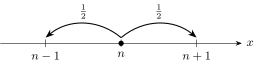
A drunk man is walking along the integer line. He starts at the origin, X0=0X_0 = 0. At each step, independently of everything before, he moves one unit right with probability 12\tfrac12 or one unit left with probability 12\tfrac12. Let XnX_n be his location after nn steps.

Number line with the walker at n and arrows to n − 1 and n + 1, each labeled probability 1/2

Questions: What is E[Xn]\EE[X_n]? What is E[Xn2]\EE[X_n^2], and how far from the origin is he typically?

Write the (n+1)(n+1)-th step using two indicator random variables,

1+(n+1)={1if step n+1 is +1,0otherwise,1−(n+1)={1if step n+1 is −1,0otherwise.\mathbf{1}_{+}^{(n+1)} = \begin{cases} 1 & \text{if step } n+1 \text{ is } +1, \\ 0 & \text{otherwise,} \end{cases} \qquad \mathbf{1}_{-}^{(n+1)} = \begin{cases} 1 & \text{if step } n+1 \text{ is } -1, \\ 0 & \text{otherwise.} \end{cases}

Exactly one of them equals 11, so the step is 1+(n+1)−1−(n+1)∈{+1,−1}\mathbf{1}_{+}^{(n+1)} - \mathbf{1}_{-}^{(n+1)} \in \{+1, -1\}, and

Xn+1=Xn+1+(n+1)−1−(n+1).(5.19)X_{n+1} = X_n + \mathbf{1}_{+}^{(n+1)} - \mathbf{1}_{-}^{(n+1)}. \tag{5.19}

Notation. An indicator only takes the values 00 and 11, so a step of −1-1 is written by subtracting the indicator 1−(n+1)\mathbf{1}_{-}^{(n+1)}. The superscript (n+1)(n+1) records that each step is a fresh, independent coin flip. Similarly, the location XnX_n and the step taken at time nn are different random variables, so we keep separate names for them.

The mean: 𝔼[Xₙ] = 0 for all n

Take expectations in (5.19). By linearity, and since E[1±(n+1)]=P(step is ±1)=12\EE[\mathbf{1}_{\pm}^{(n+1)}] = \PP(\text{step is } \pm 1) = \tfrac12,

E[Xn+1]=E[Xn]+E[1+(n+1)]−E[1−(n+1)]=E[Xn]+12−12=E[Xn].(5.20)\EE[X_{n+1}] = \EE[X_n] + \EE\bigl[\mathbf{1}_{+}^{(n+1)}\bigr] - \EE\bigl[\mathbf{1}_{-}^{(n+1)}\bigr] = \EE[X_n] + \tfrac12 - \tfrac12 = \EE[X_n]. \tag{5.20}

So one step never changes the expected location.

Theorem 5.3 (Mean of the symmetric random walk)

For every n≥0n \ge 0, E[Xn]=0\EE[X_n] = 0.

Proof.

By induction on nn. Base case: X0=0X_0 = 0 is a constant, so E[X0]=0\EE[X_0] = 0. Inductive step: suppose E[Xn]=0\EE[X_n] = 0. By (5.20), E[Xn+1]=E[Xn]=0\EE[X_{n+1}] = \EE[X_n] = 0. Unrolled, this is just a chain of equalities:

E[Xn]=E[Xn−1]=E[Xn−2]=⋯=E[X1]=E[X0]=0.\EE[X_n] = \EE[X_{n-1}] = \EE[X_{n-2}] = \cdots = \EE[X_1] = \EE[X_0] = 0.

Two more ways to see it.

  1. Sum of steps. Let ξi∈{+1,−1}\xi_i \in \{+1, -1\} be the ii-th step, so Xn=ξ1+ξ2+⋯+ξnX_n = \xi_1 + \xi_2 + \cdots + \xi_n. Each step has mean E[ξi]=(+1)⋅12+(−1)⋅12=0\EE[\xi_i] = (+1)\cdot\tfrac12 + (-1)\cdot\tfrac12 = 0, and by linearity E[Xn]=∑i=1nE[ξi]=0\EE[X_n] = \sum_{i=1}^n \EE[\xi_i] = 0.
  2. Symmetry. Flipping the direction of every step turns the walk XnX_n into −Xn-X_n, and since left and right are equally likely, the flipped walk has exactly the same distribution. So E[Xn]=E[−Xn]=−E[Xn]\EE[X_n] = \EE[-X_n] = -\EE[X_n], which forces E[Xn]=0\EE[X_n] = 0.

A zero mean does not mean the walker stays near the origin. He drifts away, but is equally likely to drift left or right, so the drifts cancel in the average. To measure how far he wanders, we need the second moment.

The second moment: 𝔼[Xₙ²] = n

Suppose Xn=kX_n = k. The next step is ±1\pm 1 with probability 12\tfrac12 each, independent of the past, so

P(Xn+12=(k+1)2∣Xn=k)=12,P(Xn+12=(k−1)2∣Xn=k)=12.\PP\bigl(X_{n+1}^2 = (k+1)^2 \mid X_n = k\bigr) = \tfrac12, \qquad \PP\bigl(X_{n+1}^2 = (k-1)^2 \mid X_n = k\bigr) = \tfrac12.

These are the same two equally likely moves (k→k+1k \to k+1 and k→k−1k \to k-1), just with the resulting location squared. Therefore

E[Xn+12∣Xn=k]=12(k+1)2+12(k−1)2=12(k2+2k+1)+12(k2−2k+1)=k2+1.\begin{aligned} \EE\bigl[X_{n+1}^2 \mid X_n = k\bigr] &= \tfrac12 (k+1)^2 + \tfrac12 (k-1)^2 \\ &= \tfrac12 (k^2 + 2k + 1) + \tfrac12 (k^2 - 2k + 1) \\ &= k^2 + 1. \end{aligned}

The edge case k=0k = 0. When k=0k = 0, (k+1)2=(k−1)2=1(k+1)^2 = (k-1)^2 = 1, so the two events above are the same event, which has probability 11 (not 12\tfrac12). The computation of E[Xn+12∣Xn=0]\EE[X_{n+1}^2 \mid X_n = 0] is still correct, because we are really averaging over the two moves: 12⋅1+12⋅1=1=02+1\tfrac12 \cdot 1 + \tfrac12 \cdot 1 = 1 = 0^2 + 1.

We found g(k)=E[Xn+12∣Xn=k]=k2+1g(k) = \EE[X_{n+1}^2 \mid X_n = k] = k^2 + 1. Replacing the value kk by the random variable XnX_n (the “pattern matching” step, exactly as in E[X∣N]=N/2\EE[X \mid N] = N/2):

E[Xn+12∣Xn]=Xn2+1.\EE\bigl[X_{n+1}^2 \mid X_n\bigr] = X_n^2 + 1.

By the law of iterated expectation,

E[Xn+12]=E[E[Xn+12∣Xn]](law of iterated expectation)=E[Xn2+1]=1+E[Xn2].(linearity)\begin{aligned} \EE\bigl[X_{n+1}^2\bigr] &= \EE\bigl[\EE[X_{n+1}^2 \mid X_n]\bigr] && \text{(law of iterated expectation)} \\ &= \EE\bigl[X_n^2 + 1\bigr] \\ &= 1 + \EE\bigl[X_n^2\bigr]. && \text{(linearity)} \end{aligned}

Each step adds exactly 11 to the second moment, starting from E[X02]=0\EE[X_0^2] = 0:

E[X02]=0,E[X12]=1,E[X22]=2,…⟹E[Xn2]=n,\EE[X_0^2] = 0, \quad \EE[X_1^2] = 1, \quad \EE[X_2^2] = 2, \quad \ldots \quad\Longrightarrow\quad \EE[X_n^2] = n,

(formally, by induction exactly as for the mean). In particular E[Xn+12]=1+n\EE[X_{n+1}^2] = 1 + n.

Theorem 5.4 (Spread of the symmetric random walk)

For every n≥0n \ge 0,

Var⁡(Xn)=E[Xn2]−(E[Xn])2=n−02=n,soσXn=n.\Var(X_n) = \EE[X_n^2] - (\EE[X_n])^2 = n - 0^2 = n, \qquad\text{so}\qquad \sigma_{X_n} = \sqrt{n}.

Cross-check with Lecture 4. With Xn=ξ1+⋯+ξnX_n = \xi_1 + \cdots + \xi_n and independent steps, each step has Var⁡(ξi)=E[ξi2]−02=1\Var(\xi_i) = \EE[\xi_i^2] - 0^2 = 1 (since ξi2=1\xi_i^2 = 1 always). The variance of a sum of independent random variables is the sum of the variances, so Var⁡(Xn)=n\Var(X_n) = n. Same answer, no conditioning needed.

Key takeaway. The walker’s expected position is 00 forever, but his typical distance from the origin is n\sqrt{n}: after 10,00010{,}000 steps he is typically about 100100 units away. This n\sqrt{n} growth is the signature of diffusion, and it reappears throughout the course.

Conditional Variance and the Law of Total Variance

Definition 5.1 (Conditional variance)

For yy with P(Y=y)>0\PP(Y = y) > 0, the conditional variance of XX given Y=yY = y is the variance of the conditional distribution of XX:

Var⁡(X∣Y=y)≜E[(X−E[X∣Y=y])2∣Y=y]=E[X2∣Y=y]−(E[X∣Y=y])2.\Var(X \mid Y = y) \triangleq \EE\Bigl[\bigl(X - \EE[X \mid Y = y]\bigr)^2 \Bigm| Y = y\Bigr] = \EE[X^2 \mid Y = y] - \bigl(\EE[X \mid Y = y]\bigr)^2.

This is a number for each yy, so Var⁡(X∣Y)\Var(X \mid Y), obtained by replacing yy with YY, is a function of YY, and hence a random variable.

(The second form follows exactly as in Lecture 3, applied to the conditional distribution of XX given Y=yY = y.)

Theorem 5.5 (Law of total variance)

For random variables X,YX, Y with E[X2]<∞\EE[X^2] < \infty,

Var⁡(X)=E[Var⁡(X∣Y)]+Var⁡(E[X∣Y]).\Var(X) = \EE\bigl[\Var(X \mid Y)\bigr] + \Var\bigl(\EE[X \mid Y]\bigr).
Proof.

Abbreviate μ(Y)=E[X∣Y]\mu(Y) = \EE[X \mid Y], so that Var⁡(X∣Y)=E[X2∣Y]−μ(Y)2\Var(X \mid Y) = \EE[X^2 \mid Y] - \mu(Y)^2.

Take expectations and use the tower rule on E[X2∣Y]\EE[X^2 \mid Y]:

E[Var⁡(X∣Y)]=E[E[X2∣Y]]−E[μ(Y)2]=E[X2]−E[μ(Y)2].\EE\bigl[\Var(X \mid Y)\bigr] = \EE\bigl[\EE[X^2 \mid Y]\bigr] - \EE\bigl[\mu(Y)^2\bigr] = \EE[X^2] - \EE\bigl[\mu(Y)^2\bigr].

Next, μ(Y)\mu(Y) is a random variable; apply the variance formula to it, and use the tower rule on its mean, E[μ(Y)]=E[E[X∣Y]]=E[X]\EE[\mu(Y)] = \EE[\EE[X\mid Y]] = \EE[X]:

Var⁡(μ(Y))=E[μ(Y)2]−(E[μ(Y)])2=E[μ(Y)2]−(E[X])2.\Var\bigl(\mu(Y)\bigr) = \EE\bigl[\mu(Y)^2\bigr] - \bigl(\EE[\mu(Y)]\bigr)^2 = \EE\bigl[\mu(Y)^2\bigr] - (\EE[X])^2.

Adding the two, the E[μ(Y)2]\EE[\mu(Y)^2] terms cancel:

E[Var⁡(X∣Y)]+Var⁡(E[X∣Y])=E[X2]−E[μ(Y)2]+E[μ(Y)2]−(E[X])2=Var⁡(X).\begin{aligned} \EE\bigl[\Var(X \mid Y)\bigr] + \Var\bigl(\EE[X \mid Y]\bigr) &= \EE[X^2] - \EE\bigl[\mu(Y)^2\bigr] + \EE\bigl[\mu(Y)^2\bigr] - (\EE[X])^2 \\ &= \Var(X). \end{aligned}

Interpretation: within-group plus between-group. Group the outcomes by the value of YY. Then E[Var⁡(X∣Y)]\EE[\Var(X \mid Y)] is the average spread within each group, and Var⁡(E[X∣Y])\Var(\EE[X \mid Y]) is the spread between the group means. Total spread is the sum of the two. Since both terms are nonnegative, Var⁡(X)≥E[Var⁡(X∣Y)]\Var(X) \ge \EE[\Var(X \mid Y)]: on average, learning YY can only reduce our uncertainty about XX.

Example 5.5 (Variance of heads in a random number of tosses)

Continue the example with N∼Geometric⁡(p)N \sim \Geom(p) and X∣N∼Binomial⁡(N,12)X \mid N \sim \Bin(N, \tfrac12). From the binomial formulas of Lecture 4,

E[X∣N]=N2,Var⁡(X∣N)=N⋅12⋅12=N4.\EE[X \mid N] = \frac{N}{2}, \qquad \Var(X \mid N) = N \cdot \tfrac12 \cdot \tfrac12 = \frac{N}{4}.

Using E[N]=1p\EE[N] = \frac1p and Var⁡(N)=1−pp2\Var(N) = \frac{1-p}{p^2}:

E[Var⁡(X∣N)]=E[N4]=14⋅1p=14p,Var⁡(E[X∣N])=Var⁡(N2)=14 Var⁡(N)=1−p4p2.\begin{aligned} \EE\bigl[\Var(X \mid N)\bigr] &= \EE\Bigl[\frac{N}{4}\Bigr] = \frac14 \cdot \frac1p = \frac{1}{4p}, \\ \Var\bigl(\EE[X \mid N]\bigr) &= \Var\Bigl(\frac{N}{2}\Bigr) = \frac14\,\Var(N) = \frac{1-p}{4p^2}. \end{aligned}

By the law of total variance,

Var⁡(X)=14p+1−p4p2=p4p2+1−p4p2=14p2.\Var(X) = \frac{1}{4p} + \frac{1-p}{4p^2} = \frac{p}{4p^2} + \frac{1-p}{4p^2} = \frac{1}{4p^2}.

Sanity check: if p=1p = 1, then N=1N = 1 and X∼Bernoulli⁡(12)X \sim \Bern(\tfrac12), whose variance is 12⋅12=14\tfrac12\cdot\tfrac12 = \tfrac14. ✓

Continuous Random Variables

Continuous random variables (CRVs) let us measure uncertainty in a principled way for quantities that vary continuously, such as velocity, time, and distance.

Coming up. Important continuous distributions include the uniform, exponential, and gamma distributions, which we develop in upcoming lectures. The exponential is the continuous analog of the geometric (Lecture 4).

Why discrete tools break. Let X∼Uniform⁡[0,1]X \sim \operatorname{Uniform}[0,1], a number chosen “uniformly at random” from [0,1][0,1]. Then:

  • P(X=x)=0\PP(X = x) = 0 for any specific number xx (there are uncountably many equally likely candidates);
  • yet P(X<12)=12\PP(X < \tfrac12) = \tfrac12.

So we cannot build probabilities by adding up point masses as we did with PMFs. Instead, we assign probabilities directly to sets that are “allowable events.”

Definition 5.2 (Allowable events (Borel sets))

The allowable events for a real-valued random variable include all intervals,

(−∞,a),[a,b],(a,b],…(-\infty, a), \qquad [a, b], \qquad (a, b], \qquad \ldots

together with everything obtainable from intervals by countable unions, countable intersections, and complements, e.g. (a,b)∪(c,d)(a, b) \cup (c, d). These are the Borel sets; they form the Borel σ\sigma-algebra from Lecture 1. In practice, any “reasonable” set is allowable.

Recall that for a discrete random variable (DRV) and a set of values BB,

P(X∈B)=∑x∈BpX(x).\PP(X \in B) = \sum_{x \in B} p_X(x).

For a CRV, the sum over points becomes an integral of a density.

Definition 5.3 (Continuous random variable and PDF)

A random variable XX is continuous if there is a function fX:R→[0,∞)f_X : \RR \to [0, \infty), called its probability density function (PDF), such that for every allowable set BB,

P(X∈B)=∫BfX(x) dx.\PP(X \in B) = \int_B f_X(x)\,dx.

A density must satisfy

fX(x)≥0   for all x,and∫−∞∞fX(x) dx=1.f_X(x) \ge 0 \;\text{ for all } x, \qquad\text{and}\qquad \int_{-\infty}^{\infty} f_X(x)\,dx = 1.

In particular, P(a≤X≤b)=∫abfX(x) dx\PP(a \le X \le b) = \int_a^b f_X(x)\,dx is the area under the density between aa and bb.

A density curve f_X(x) with the area between a and b shaded, labeled P(a ≤ X ≤ b)
Theorem 5.6 (Single points have probability zero)

If XX is continuous, then P(X=x)=0\PP(X = x) = 0 for every x∈Rx \in \RR.

Proof.

Fix xx and any δ>0\delta > 0. The event {X=x}\{X = x\} is contained in {x≤X<x+δ}\{x \le X < x + \delta\}, so

P(X=x)≤P(x≤X<x+δ)=∫xx+δfX(u) du.\PP(X = x) \le \PP(x \le X < x + \delta) = \int_x^{x+\delta} f_X(u)\,du.

(We use the dummy variable uu inside the integral so as not to confuse it with xx, which now appears in the limits.) As δ→0\delta \to 0, this is the integral of fXf_X over a shrinking interval, which tends to 00. If fXf_X is continuous at xx, we can see this explicitly: the sliver is approximately a rectangle of height fX(x)f_X(x) and width δ\delta, so the integral is ≈fX(x) δ→0\approx f_X(x)\,\delta \to 0. Since P(X=x)\PP(X = x) is smaller than a quantity that can be made arbitrarily small, P(X=x)=0\PP(X = x) = 0.

A thin sliver under the density f_X(u) between x and x + δ, with area approximately f_X(x) δ

A density is not a probability. fX(x)f_X(x) has units of probability per unit length. Wherever fXf_X is continuous,

fX(x)=lim⁡δ→0P(x≤X<x+δ)δ,i.e.P(x≤X<x+δ)≈fX(x) δ for small δ.f_X(x) = \lim_{\delta \to 0} \frac{\PP(x \le X < x + \delta)}{\delta}, \quad\text{i.e.}\quad \PP(x \le X < x + \delta) \approx f_X(x)\,\delta \text{ for small } \delta.

Don’t confuse fX(x)f_X(x) with a probability: it is a density. Only areas under fXf_X are probabilities, so fX(x)f_X(x) itself may exceed 11, as the next example shows.

Example 5.6 (An unbounded density)

Let

fX(x)={12x0<x≤1,0otherwise.f_X(x) = \begin{cases} \dfrac{1}{2\sqrt{x}} & 0 < x \le 1, \\[4pt] 0 & \text{otherwise.} \end{cases}

It is a valid PDF. Clearly fX≥0f_X \ge 0. For the total area, write 12x=12x−1/2\frac{1}{2\sqrt{x}} = \frac12 x^{-1/2} and integrate:

∫−∞∞fX(x) dx=∫0112 x−1/2 dx=12[ 2x1/2]01=[x ]01=1−0=1.\int_{-\infty}^{\infty} f_X(x)\,dx = \int_0^1 \tfrac12\, x^{-1/2}\,dx = \tfrac12 \Bigl[\, 2x^{1/2} \Bigr]_0^1 = \Bigl[\sqrt{x}\,\Bigr]_0^1 = 1 - 0 = 1.

It exceeds 11, and is even unbounded. fX(1)=12f_X(1) = \tfrac12, but fX(0.01)=12(0.1)=5f_X(0.01) = \frac{1}{2(0.1)} = 5, and fX(x)→∞f_X(x) \to \infty as x→0+x \to 0^+. Nevertheless every probability is finite, e.g. P(X≤0.01)=∫00.0112x−1/2 dx=0.01=0.1\PP(X \le 0.01) = \int_0^{0.01}\tfrac12 x^{-1/2}\,dx = \sqrt{0.01} = 0.1.

Graph of f_X(x) = 1/(2√x) on (0, 1], rising without bound as x approaches 0, with the area underneath shaded

The Cumulative Distribution Function

Definition 5.4 (Cumulative distribution function (CDF))

The cumulative distribution function of any random variable XX (discrete or continuous) is

FX(x)≜P(X≤x),x∈R.F_X(x) \triangleq \PP(X \le x), \qquad x \in \RR.

For a continuous random variable,

FX(x)=∫−∞xfX(u) du.F_X(x) = \int_{-\infty}^{x} f_X(u)\,du.
Theorem 5.7 (Properties of the CDF)

Every CDF satisfies:

  1. Nondecreasing: if x≤yx \le y then FX(x)≤FX(y)F_X(x) \le F_X(y), since {X≤x}⊆{X≤y}\{X \le x\} \subseteq \{X \le y\}.
  2. Limits: lim⁡x→−∞FX(x)=0\displaystyle\lim_{x \to -\infty} F_X(x) = 0 and lim⁡x→+∞FX(x)=1\displaystyle\lim_{x \to +\infty} F_X(x) = 1.
  3. Intervals: P(a<X≤b)=FX(b)−FX(a)\PP(a < X \le b) = F_X(b) - F_X(a), because {X≤b}\{X \le b\} is the disjoint union of {X≤a}\{X \le a\} and {a<X≤b}\{a < X \le b\}.
Theorem 5.8 (Recovering the PMF or PDF from the CDF)
  • CRV: wherever fXf_X is continuous, fX(x)=dFX(x)dx.f_X(x) = \frac{dF_X(x)}{dx}.
  • Integer-valued DRV: for every integer kk, P(X=k)=FX(k)−FX(k−1).\PP(X = k) = F_X(k) - F_X(k-1).
Proof.

CRV: FX(x)=∫−∞xfX(u) duF_X(x) = \int_{-\infty}^x f_X(u)\,du, so this is the fundamental theorem of calculus. DRV: because XX only takes integer values, there are no possible values strictly between k−1k-1 and kk. So {X≤k}\{X \le k\} is the disjoint union of {X≤k−1}\{X \le k-1\} and {X=k}\{X = k\}, giving FX(k)=FX(k−1)+P(X=k)F_X(k) = F_X(k-1) + \PP(X = k). (For a discrete random variable taking non-integer values, use the jump of FXF_X at the value instead.)

Picturing the two kinds of CDF. For an integer-valued DRV, FXF_X is a staircase. On each open interval (k−1,k)(k-1, k) there are no possible values, so no new probability accumulates and FXF_X stays flat, holding the value FX(k−1)F_X(k-1). It does not drop back to zero: all the probability collected up through k−1k-1 is still counted. At kk itself, FXF_X jumps up by exactly P(X=k)\PP(X = k). For a CRV, single points carry no probability, so FXF_X rises continuously with no jumps.

Left: the staircase CDF of an integer-valued discrete random variable, jumping by P(X = k) at k. Right: the continuous CDF of Uniform[0,1], rising linearly from 0 to 1
Corollary 5.1 (Consequences for continuous random variables)

If XX is continuous, then for all a≤ba \le b:

P(a≤X≤b)=∫abfX(x) dx=FX(b)−FX(a),\PP(a \le X \le b) = \int_a^b f_X(x)\,dx = F_X(b) - F_X(a),P(X=a)=0,P(X<a)=P(X≤a).\PP(X = a) = 0, \qquad \PP(X < a) = \PP(X \le a).

Because points do not contribute, it does not matter whether the endpoints of an interval are included: P(a<X<b)=P(a≤X<b)=P(a<X≤b)=P(a≤X≤b)\PP(a < X < b) = \PP(a \le X < b) = \PP(a < X \le b) = \PP(a \le X \le b). This is false for discrete random variables, where P(X<k)\PP(X < k) and P(X≤k)\PP(X \le k) differ by P(X=k)\PP(X = k).

Example: A Random Dart on a Disk

Example 5.7 (Random dart on the unit disk)

A dart lands uniformly at random on a disk of radius 11 (the unit circle and its interior). “Uniformly” means the probability of landing in any region is proportional to its area:

P(dart lands in region R)=Area(R)Area of full disk=Area(R)π(1)2.\PP(\text{dart lands in region } R) = \frac{\text{Area}(R)}{\text{Area of full disk}} = \frac{\text{Area}(R)}{\pi (1)^2}.

Let YY be the dart’s distance from the center. Find the PDF fY(y)f_Y(y).

Unit disk with a shaded inner disk of radius y, labeled Y ≤ y, and a dart landing inside the unit disk

It is easiest to compute FY(y)=P(Y≤y)F_Y(y) = \PP(Y \le y) first. For 0≤y≤10 \le y \le 1, the event {Y≤y}\{Y \le y\} means the dart lands in the shaded disk of radius yy:

FY(y)=P(Y≤y)=Area shadedArea full disk=πy2π(1)2=y2.F_Y(y) = \PP(Y \le y) = \frac{\text{Area shaded}}{\text{Area full disk}} = \frac{\pi y^2}{\pi (1)^2} = y^2.

Outside [0,1][0,1]: FY(y)=0F_Y(y) = 0 for y<0y < 0 (distance is never negative) and FY(y)=1F_Y(y) = 1 for y>1y > 1 (the dart is always on the disk).

Differentiating,

fY(y)=dFY(y)dy=ddy(y2)=2y,0≤y≤1,f_Y(y) = \frac{dF_Y(y)}{dy} = \frac{d}{dy}\bigl(y^2\bigr) = 2y, \qquad 0 \le y \le 1,

and fY(y)=0f_Y(y) = 0 otherwise. Check: ∫012y dy=[y2]01=1\int_0^1 2y\,dy = \bigl[y^2\bigr]_0^1 = 1. ✓

By the CDF,

P(Y∈(0.5,0.6))=FY(0.6)−FY(0.5)=0.62−0.52=0.36−0.25=0.11.\PP\bigl(Y \in (0.5, 0.6)\bigr) = F_Y(0.6) - F_Y(0.5) = 0.6^2 - 0.5^2 = 0.36 - 0.25 = 0.11.

Or, equivalently, by the PDF: ∫0.50.62y dy=[y2]0.50.6=0.11\int_{0.5}^{0.6} 2y\,dy = \bigl[y^2\bigr]_{0.5}^{0.6} = 0.11.

Three traps in this example.

  1. YY is not uniform on [0,1][0,1]. The dart’s position is uniform on the disk, but its distance from the center is not: the density 2y2y grows with yy, because there is more area at larger radii. The ring 0.5<Y<0.60.5 < Y < 0.6 has probability 0.110.11, while the same-width band 0<Y<0.10 < Y < 0.1 near the center has only 0.12=0.010.1^2 = 0.01.
  2. Don’t stop at the CDF. y2y^2 is FYF_Y, not fYf_Y; the PDF requires the extra differentiation step.
  3. 1πr2\frac{1}{\pi r^2} is a 2-D density. The constant 1πr2\frac{1}{\pi r^2} (here 1π\frac1\pi) is the density of the dart’s position per unit area. It is not fYf_Y, which is a density per unit length along the radius.

The CDF method. This “CDF first, then differentiate” strategy is the standard way to find the density of a function of a random variable.

Example: Meeting at Random Times

Not finished in lecture. We ran out of time after posing this problem. The full solution is given below.

Example 5.8 (Will A and B meet?)

AA and BB each arrive at a meeting spot at a uniformly random time between 4:00 pm and 5:00 pm, independently of each other. Whoever arrives first waits 1010 minutes and then leaves. What is P(A and B meet)\PP(A \text{ and } B \text{ meet})?

Setup. Measure time in minutes after 4:00 pm, so AA and BB are independent Uniform⁡[0,60]\operatorname{Uniform}[0, 60] random variables. The pair (A,B)(A, B) is a point in the 60×6060 \times 60 square [0,60]2[0,60]^2. Because AA and BB are independent and each uniform, the point (A,B)(A, B) is uniform on the square:

P((A,B)∈R)=Area(R)60×60=Area(R)3600.\PP\bigl((A, B) \in R\bigr) = \frac{\text{Area}(R)}{60 \times 60} = \frac{\text{Area}(R)}{3600}.

(Joint distributions of several continuous random variables are developed formally in upcoming lectures; this “probability == area fraction” rule is the two-dimensional version of the uniform distribution, exactly as in the dart example.)

When do they meet? Whoever arrives first waits 1010 minutes, so they meet exactly when their arrival times differ by at most 1010 minutes:

{A and B meet}={∣A−B∣≤10}.\{A \text{ and } B \text{ meet}\} = \bigl\{|A - B| \le 10\bigr\}.

This is the shaded diagonal band in the figure below.

The 60 by 60 square of arrival times (A, B), with the diagonal band |A − B| ≤ 10 shaded as the meeting region and two corner triangles where they miss each other

Compute the complement. The two blue corner regions, where they miss each other, are right triangles:

  • {A−B>10}\{A - B > 10\}: AA arrives more than 1010 minutes after BB, so BB has already left. The triangle has vertices (10,0),(60,0),(60,50)(10,0), (60,0), (60,50) and legs of length 5050.
  • {B−A>10}\{B - A > 10\}: the mirror image, with vertices (0,10),(0,60),(50,60)(0,10), (0,60), (50,60), also with legs of length 5050.

Each triangle has area 12⋅50⋅50=1250\tfrac12 \cdot 50 \cdot 50 = 1250, so together they cover 25002500 out of 36003600:

P(miss)=2⋅12503600=25003600=2536.\PP(\text{miss}) = \frac{2 \cdot 1250}{3600} = \frac{2500}{3600} = \frac{25}{36}.

Therefore

P(A and B meet)=1−2536=1136≈0.306.\PP(A \text{ and } B \text{ meet}) = 1 - \frac{25}{36} = \frac{11}{36} \approx 0.306.

Equivalently, the band has area 3600−2500=11003600 - 2500 = 1100, and 11003600=1136\frac{1100}{3600} = \frac{11}{36}.

Checks and generalization.

  1. Boundaries don’t matter. The lines ∣A−B∣=10|A - B| = 10 have zero area, so it makes no difference whether “waits 1010 minutes” includes the endpoint. This is the two-dimensional version of P(X<a)=P(X≤a)\PP(X < a) = \PP(X \le a).
  2. General formula. With a window of length TT and waiting time w≤Tw \le T, the same picture gives P(meet)=1−(1−wT)2.\PP(\text{meet}) = 1 - \Bigl(1 - \frac{w}{T}\Bigr)^2. With w=10w = 10, T=60T = 60: 1−(5/6)2=11/361 - (5/6)^2 = 11/36. Sanity checks: w=0w = 0 gives 00 (they must arrive at the exact same instant), and w=Tw = T gives 11.

Lecture 7: The Gaussian Distribution, Derived Distributions, and Order Statistics

EECS 126 (UC Berkeley) · Spring 2026 · February 10, 2026

Reading: Bertsekas & Tsitsiklis, §3.3, §4.1.

These are my personal notes from Professor Kannan Ramchandran’s EECS 126 (Probability and Random Processes) course at UC Berkeley.

Topics: the Gaussian distribution, change of variables (derived distributions), and order statistics.

The Gaussian Distribution

Definition 7.1 (Gaussian (normal) distribution)

X∼N(μ,σ2)X \sim \mathcal{N}(\mu, \sigma^2), with μ∈R\mu \in \RR and σ>0\sigma > 0, if

fX(x)=12π σ e−(x−μ)2/2σ2,x∈R.f_X(x) = \frac{1}{\sqrt{2\pi}\,\sigma}\, e^{-(x-\mu)^2/2\sigma^2}, \qquad x \in \RR.

The standard normal is Z∼N(0,1)Z \sim \mathcal{N}(0, 1):

fZ(z)=12π e−z2/2,z∈R.(7.2)f_Z(z) = \frac{1}{\sqrt{2\pi}}\, e^{-z^2/2}, \qquad z \in \RR. \tag{7.2}

The constant 12π\frac{1}{\sqrt{2\pi}} is the normalization factor that makes ∫−∞∞fZ(z) dz=1\int_{-\infty}^{\infty} f_Z(z)\,dz = 1.

Definition 7.2 (Standard normal CDF)
Φ(z)≜P(Z≤z)=∫−∞z12π e−u2/2 du.\Phi(z) \triangleq \PP(Z \le z) = \int_{-\infty}^{z} \frac{1}{\sqrt{2\pi}}\, e^{-u^2/2}\, du.

uu is a dummy variable of integration; zz appears only in the upper limit. Φ\Phi has no closed form, so its values are read from a table.

Theorem 7.1 (Key Gaussian integral)

For every α>0\alpha > 0,

∫−∞∞e−αx2/2 dx=2πα,\int_{-\infty}^{\infty} e^{-\alpha x^2/2}\, dx = \sqrt{\frac{2\pi}{\alpha}},

or equivalently

I(α)≜12π∫−∞∞e−αx2/2 dx=1α=α−1/2.(7.5)I(\alpha) \triangleq \frac{1}{\sqrt{2\pi}} \int_{-\infty}^{\infty} e^{-\alpha x^2/2}\, dx = \frac{1}{\sqrt{\alpha}} = \alpha^{-1/2}. \tag{7.5}
Proof.

Substitute u=α xu = \sqrt{\alpha}\,x, so du=α dxdu = \sqrt{\alpha}\,dx and αx2=u2\alpha x^2 = u^2:

∫−∞∞e−αx2/2 dx=∫−∞∞e−u2/2 duα=1α∫−∞∞e−u2/2 du=1α⋅2π,\int_{-\infty}^{\infty} e^{-\alpha x^2/2}\, dx = \int_{-\infty}^{\infty} e^{-u^2/2}\, \frac{du}{\sqrt{\alpha}} = \frac{1}{\sqrt{\alpha}} \int_{-\infty}^{\infty} e^{-u^2/2}\, du = \frac{1}{\sqrt{\alpha}} \cdot \sqrt{2\pi},

where the last step uses ∫−∞∞12πe−u2/2 du=1\int_{-\infty}^{\infty} \frac{1}{\sqrt{2\pi}} e^{-u^2/2}\,du = 1 from (7.2). Dividing by 2π\sqrt{2\pi} gives (7.5).

Mean and Variance of the Standard Normal

Theorem 7.2 (Standard normal moments)

If Z∼N(0,1)Z \sim \mathcal{N}(0,1), then E[Z]=0\EE[Z] = 0 and Var⁡(Z)=1\Var(Z) = 1.

Proof of 𝔼[Z] = 0. E[Z]=∫−∞∞z fZ(z) dz=∫−∞∞12π z e−z2/2 dz.\EE[Z] = \int_{-\infty}^{\infty} z\, f_Z(z)\, dz = \int_{-\infty}^{\infty} \frac{1}{\sqrt{2\pi}}\, z\, e^{-z^2/2}\, dz.

The integrand g(z)=z e−z2/2g(z) = z\,e^{-z^2/2} is odd, g(−z)=−g(z)g(-z) = -g(z), so the two halves cancel:

∫0∞z e−z2/2 dz=[−e−z2/2]0∞=0−(−1)=1,∫−∞0z e−z2/2 dz=[−e−z2/2]−∞0=−1−0=−1,\begin{aligned} \int_{0}^{\infty} z\, e^{-z^2/2}\, dz &= \Bigl[-e^{-z^2/2}\Bigr]_0^{\infty} = 0 - (-1) = 1, \\ \int_{-\infty}^{0} z\, e^{-z^2/2}\, dz &= \Bigl[-e^{-z^2/2}\Bigr]_{-\infty}^{0} = -1 - 0 = -1, \end{aligned}

and therefore E[Z]=12π(1−1)=0\EE[Z] = \frac{1}{\sqrt{2\pi}}(1 - 1) = 0.

Proof of Var(Z) = 1.

Differentiate e−αx2/2e^{-\alpha x^2/2} with respect to α\alpha:

ddα(e−αx2/2)=−x22 e−αx2/2⟹x2e−αx2/2=−2 ddα(e−αx2/2).\frac{d}{d\alpha}\Bigl(e^{-\alpha x^2/2}\Bigr) = -\frac{x^2}{2}\, e^{-\alpha x^2/2} \quad\Longrightarrow\quad x^2 e^{-\alpha x^2/2} = -2\, \frac{d}{d\alpha}\Bigl(e^{-\alpha x^2/2}\Bigr).

Then

E[Z2]=∫−∞∞x2 12π e−x2/2 dx=[∫−∞∞12π x2e−αx2/2 dx]α=1=[∫−∞∞−22π ddα(e−αx2/2) dx]α=1=[−2 ddα(12π∫−∞∞e−αx2/2 dx)]α=1(Leibniz rule)=[−2 ddα I(α)]α=1=[−2 ddα α−1/2]α=1by (7.5)=[−2(−12 α−3/2)]α=1=[α−3/2]α=1=[1α3]α=1=1.\begin{aligned} \EE[Z^2] &= \int_{-\infty}^{\infty} x^2\, \frac{1}{\sqrt{2\pi}}\, e^{-x^2/2}\, dx \\ &= \left[\int_{-\infty}^{\infty} \frac{1}{\sqrt{2\pi}}\, x^2 e^{-\alpha x^2/2}\, dx\right]_{\alpha=1} \\ &= \left[\int_{-\infty}^{\infty} \frac{-2}{\sqrt{2\pi}}\, \frac{d}{d\alpha}\Bigl(e^{-\alpha x^2/2}\Bigr)\, dx\right]_{\alpha=1} \\ &= \left[-2\, \frac{d}{d\alpha}\left(\frac{1}{\sqrt{2\pi}} \int_{-\infty}^{\infty} e^{-\alpha x^2/2}\, dx\right)\right]_{\alpha=1} && \text{(Leibniz rule)} \\ &= \left[-2\, \frac{d}{d\alpha}\, I(\alpha)\right]_{\alpha=1} = \left[-2\, \frac{d}{d\alpha}\, \alpha^{-1/2}\right]_{\alpha=1} && \text{by (7.5)} \\ &= \left[-2 \left(-\tfrac12\, \alpha^{-3/2}\right)\right]_{\alpha=1} = \left[\alpha^{-3/2}\right]_{\alpha=1} = \left[\frac{1}{\sqrt{\alpha^3}}\right]_{\alpha=1} = 1. \end{aligned}

The Leibniz rule (differentiation under the integral sign) justifies moving ddα\frac{d}{d\alpha} outside the integral. Finally,

Var⁡(Z)=E[Z2]−(E[Z])2=1−02=1.\Var(Z) = \EE[Z^2] - (\EE[Z])^2 = 1 - 0^2 = 1.

Why only α=1\alpha = 1? I was confused why we set α=1\alpha = 1, and whether it could be something else. The identity I(α)=α−1/2I(\alpha) = \alpha^{-1/2} holds for every α>0\alpha > 0, so II is a function of α\alpha that we can differentiate, and differentiating in α\alpha is what produces the factor x2x^2. We set α=1\alpha = 1 only after differentiating, because the standard normal has e−x2/2e^{-x^2/2}, i.e. α=1\alpha = 1. Setting α=1\alpha = 1 first would leave the constant I(1)=1I(1) = 1, whose derivative is 00.

Cross-check by integration by parts. With u=xu = x and dv=12π xe−x2/2 dxdv = \frac{1}{\sqrt{2\pi}}\, x e^{-x^2/2}\,dx, so v=−12π e−x2/2v = -\frac{1}{\sqrt{2\pi}}\, e^{-x^2/2}:

E[Z2]=[−x2π e−x2/2]−∞∞+∫−∞∞12π e−x2/2 dx=0+1=1.\EE[Z^2] = \left[-\frac{x}{\sqrt{2\pi}}\, e^{-x^2/2}\right]_{-\infty}^{\infty} + \int_{-\infty}^{\infty} \frac{1}{\sqrt{2\pi}}\, e^{-x^2/2}\, dx = 0 + 1 = 1.

Linear Transformations of Gaussians

Theorem 7.3 (Shifting and scaling a standard normal)

If Z∼N(0,1)Z \sim \mathcal{N}(0,1), σ>0\sigma > 0, and X=σZ+μX = \sigma Z + \mu, then X∼N(μ,σ2)X \sim \mathcal{N}(\mu, \sigma^2).

Proof.

Start with the CDF of XX. Since σ>0\sigma > 0, dividing by σ\sigma preserves the inequality:

FX(x)=P(X≤x)=P(σZ+μ≤x)=P(Z≤x−μσ)=FZ(z),z=x−μσ.F_X(x) = \PP(X \le x) = \PP(\sigma Z + \mu \le x) = \PP\left(Z \le \frac{x - \mu}{\sigma}\right) = F_Z(z), \qquad z = \frac{x - \mu}{\sigma}.

Differentiate with the chain rule, using dzdx=ddx(xσ−μσ)=1σ\frac{dz}{dx} = \frac{d}{dx}\left(\frac{x}{\sigma} - \frac{\mu}{\sigma}\right) = \frac{1}{\sigma}:

fX(x)=ddxFX(x)=ddxFZ(z)=fZ(z) dzdx=12π e−z2/2⋅1σ=12π σ e−(x−μ)2/2σ2.\begin{aligned} f_X(x) = \frac{d}{dx} F_X(x) = \frac{d}{dx} F_Z(z) = f_Z(z)\, \frac{dz}{dx} &= \frac{1}{\sqrt{2\pi}}\, e^{-z^2/2} \cdot \frac{1}{\sigma} \\ &= \frac{1}{\sqrt{2\pi}\,\sigma}\, e^{-(x-\mu)^2/2\sigma^2}. \end{aligned}

Is fZ(z)⋅1σf_Z(z) \cdot \frac{1}{\sigma} already the answer? I was unsure whether the line fX(x)=12πe−z2/2⋅1σf_X(x) = \frac{1}{\sqrt{2\pi}} e^{-z^2/2} \cdot \frac{1}{\sigma} was correct. It is: substituting z=x−μσz = \frac{x-\mu}{\sigma} gives exactly the N(μ,σ2)\mathcal{N}(\mu, \sigma^2) density. The factor 1σ\frac{1}{\sigma} in front comes from dzdx\frac{dz}{dx}.

Should μ\mu and σ\sigma have a subscript ZZ? I was also confused about this. No: ZZ always has mean 00 and variance 11. Here μ\mu and σ\sigma are the shift and scale applied to ZZ, and they become the mean and standard deviation of XX: E[X]=σ E[Z]+μ=μ\EE[X] = \sigma\,\EE[Z] + \mu = \mu and Var⁡(X)=σ2Var⁡(Z)=σ2\Var(X) = \sigma^2 \Var(Z) = \sigma^2. If anything, they are μX\mu_X and σX\sigma_X.

Corollary 7.1 (Standardization)

If X∼N(μ,σ2)X \sim \mathcal{N}(\mu, \sigma^2), then Z=X−μσ∼N(0,1)Z = \dfrac{X - \mu}{\sigma} \sim \mathcal{N}(0, 1), and

FX(x)=Φ ⁣(x−μσ).F_X(x) = \Phi\!\left(\frac{x - \mu}{\sigma}\right).

Symmetry of Φ and Standardization

Theorem 7.4 (Symmetry of the standard normal CDF)

For every y∈Ry \in \RR,

Φ(−y)=1−Φ(y).\Phi(-y) = 1 - \Phi(y).

So a table only needs Φ(y)\Phi(y) for y≥0y \ge 0.

Proof.

fZf_Z is even: fZ(−v)=fZ(v)f_Z(-v) = f_Z(v). Substitute u=−vu = -v, du=−dvdu = -dv:

Φ(−y)=∫−∞−yfZ(u) du=∫∞yfZ(−v) (−dv)=∫y∞fZ(v) dv=P(Z≥y)=1−P(Z<y)=1−Φ(y),\begin{aligned} \Phi(-y) = \int_{-\infty}^{-y} f_Z(u)\, du &= \int_{\infty}^{y} f_Z(-v)\,(-dv) = \int_{y}^{\infty} f_Z(v)\, dv \\ &= \PP(Z \ge y) = 1 - \PP(Z < y) = 1 - \Phi(y), \end{aligned}

using P(Z<y)=P(Z≤y)\PP(Z < y) = \PP(Z \le y) for a continuous random variable.

Standard normal density with equal shaded tails: the left tail below −y is Φ(−y) and the right tail above y is 1 − Φ(y)
Example 7.1 (Annual rainfall)

The annual rainfall in a city is X∼N(60,202)X \sim \mathcal{N}(60, 20^2), in inches. Find P(X>80)\PP(X > 80).

Standardize with Z=X−6020∼N(0,1)Z = \frac{X - 60}{20} \sim \mathcal{N}(0,1):

P(X>80)=P(X−6020>80−6020)=P(X−6020>1)=P(Z>1)=1−P(Z≤1)=1−Φ(1)=1−0.8413=0.1587.\begin{aligned} \PP(X > 80) &= \PP\left(\frac{X - 60}{20} > \frac{80 - 60}{20}\right) \\ &= \PP\left(\frac{X - 60}{20} > 1\right) = \PP(Z > 1) \\ &= 1 - \PP(Z \le 1) = 1 - \Phi(1) = 1 - 0.8413 = 0.1587. \end{aligned}
Standard normal density with the right tail above z = 1 shaded, labeled P(Z > 1)

Why 1−Φ(1)1 - \Phi(1)? I was confused why the answer is 1−Φ(1)1 - \Phi(1) rather than Φ(1)\Phi(1). Φ(1)\Phi(1) is the area to the left of 11; P(Z>1)\PP(Z > 1) is the area to the right, which is its complement.

Sums of Independent Gaussians

Theorem 7.5 (Sum of independent Gaussians)

If X∼N(μX,σX2)X \sim \mathcal{N}(\mu_X, \sigma_X^2) and Y∼N(μY,σY2)Y \sim \mathcal{N}(\mu_Y, \sigma_Y^2) are independent, then

X+Y∼N(μX+μY,  σX2+σY2).X + Y \sim \mathcal{N}\bigl(\mu_X + \mu_Y,\; \sigma_X^2 + \sigma_Y^2\bigr).

The parameters follow from Lecture 4: E[X+Y]=E[X]+E[Y]=μX+μY\EE[X+Y] = \EE[X] + \EE[Y] = \mu_X + \mu_Y, and by independence Var⁡(X+Y)=Var⁡(X)+Var⁡(Y)=σX2+σY2\Var(X+Y) = \Var(X) + \Var(Y) = \sigma_X^2 + \sigma_Y^2. The content of the theorem is that X+YX + Y is again Gaussian. This can be shown with a convolution, or in one line with moment generating functions.

Proof: MGF proof TBD in a later lecture.

Theorem 7.6 (Converse)

If XX and YY are independent and X+YX + Y is Gaussian, then XX and YY are each Gaussian (allowing a constant, i.e. variance 00).

This direction is much harder; its proof is beyond the scope of this course.

Derived Distributions

Given XX with known density fXf_X and Y=g(X)Y = g(X), find fYf_Y.

Theorem 7.7 (CDF method)
FY(y)=P(Y≤y)=P(g(X)≤y)=P(X∈{x:g(x)≤y})=∫{x : g(x)≤y}fX(x) dx,F_Y(y) = \PP(Y \le y) = \PP\bigl(g(X) \le y\bigr) = \PP\bigl(X \in \{x : g(x) \le y\}\bigr) = \int_{\{x \,:\, g(x) \le y\}} f_X(x)\, dx,

and then

fY(y)=dFY(y)dy.f_Y(y) = \frac{dF_Y(y)}{dy}.

If gg is strictly increasing, {x:g(x)≤y}={x≤g−1(y)}\{x : g(x) \le y\} = \{x \le g^{-1}(y)\}, so FY(y)=FX(g−1(y))F_Y(y) = F_X\bigl(g^{-1}(y)\bigr). If gg is strictly decreasing, the inequality flips: {x:g(x)≤y}={x≥g−1(y)}\{x : g(x) \le y\} = \{x \ge g^{-1}(y)\}, so FY(y)=1−FX(g−1(y))F_Y(y) = 1 - F_X\bigl(g^{-1}(y)\bigr).

Corollary 7.2 (Monotone change of variables)

If gg is strictly monotone and differentiable, then

fY(y)=fX(g−1(y))∣d g−1(y)dy∣.(7.21)f_Y(y) = f_X\bigl(g^{-1}(y)\bigr) \left| \frac{d\, g^{-1}(y)}{dy} \right|. \tag{7.21}
Proof.

Increasing gg: ddyFX(g−1(y))=fX(g−1(y))dg−1(y)dy\frac{d}{dy} F_X(g^{-1}(y)) = f_X(g^{-1}(y)) \frac{d g^{-1}(y)}{dy}, with dg−1(y)dy>0\frac{d g^{-1}(y)}{dy} > 0. Decreasing gg: ddy[1−FX(g−1(y))]=−fX(g−1(y))dg−1(y)dy\frac{d}{dy}\bigl[1 - F_X(g^{-1}(y))\bigr] = -f_X(g^{-1}(y)) \frac{d g^{-1}(y)}{dy}, with dg−1(y)dy<0\frac{d g^{-1}(y)}{dy} < 0. In both cases the result is (7.21).

For X=σZ+μX = \sigma Z + \mu: g−1(x)=x−μσg^{-1}(x) = \frac{x-\mu}{\sigma} and dg−1(x)dx=1σ\frac{d g^{-1}(x)}{dx} = \frac{1}{\sigma}, which is the factor 1σ\frac{1}{\sigma} found in Section 7.3.

Example 7.2 (Square root of a uniform)

Let X∼Uniform⁡[0,1]X \sim \operatorname{Uniform}[0,1] and Y=XY = \sqrt{X}. For 0≤y≤10 \le y \le 1, since x\sqrt{x} is increasing on [0,1][0,1] and both sides are nonnegative,

FY(y)=P(Y≤y)=P(X≤y)=P(X≤y2)=FX(y2)=∫0y21 dx=[x]0y2=y2−0=y2,F_Y(y) = \PP(Y \le y) = \PP(\sqrt{X} \le y) = \PP(X \le y^2) = F_X(y^2) = \int_0^{y^2} 1\, dx = \Bigl[x\Bigr]_0^{y^2} = y^2 - 0 = y^2,

with FY(y)=0F_Y(y) = 0 for y<0y < 0 and FY(y)=1F_Y(y) = 1 for y>1y > 1. Differentiating,

fY(y)=ddyFY(y)=ddy(y2)=2y,0≤y≤1.f_Y(y) = \frac{d}{dy} F_Y(y) = \frac{d}{dy}\bigl(y^2\bigr) = 2y, \qquad 0 \le y \le 1.

Check with (7.21): g−1(y)=y2g^{-1}(y) = y^2, dg−1(y)dy=2y\frac{d g^{-1}(y)}{dy} = 2y, fX(y2)=1f_X(y^2) = 1, so fY(y)=1⋅2y=2yf_Y(y) = 1 \cdot 2y = 2y.

Graph of y = √x on [0, 1]

Y=XY = \sqrt{X} has the same density 2y2y as the distance of a random dart from the center of the unit disk (Lecture 5).

Order Statistics

Let X1,X2,…,XnX_1, X_2, \ldots, X_n be i.i.d. samples with common density fXf_X and CDF FXF_X.

Definition 7.3 (Order statistics)
X(k)≜the k-th smallest of X1,X2,…,Xn,k=1,…,n.X^{(k)} \triangleq \text{the } k\text{-th smallest of } X_1, X_2, \ldots, X_n, \qquad k = 1, \ldots, n.

In particular X(1)=min⁡iXiX^{(1)} = \min_i X_i and X(n)=max⁡iXiX^{(n)} = \max_i X_i.

Example 7.3 (Ordering three samples)

n=3n = 3, Xi∼Uniform⁡(0,1)X_i \sim \operatorname{Uniform}(0,1), observed (X1,X2,X3)=(0.3, 0.8, 0.4)(X_1, X_2, X_3) = (0.3,\, 0.8,\, 0.4). Then

X(1)=0.3,X(2)=0.4,X(3)=0.8.X^{(1)} = 0.3, \qquad X^{(2)} = 0.4, \qquad X^{(3)} = 0.8.

Question: what is fX(k)(x)f_{X^{(k)}}(x), the density of X(k)X^{(k)}?

By the definition of a density,

P(X(k)∈(x,x+dx))≈fX(k)(x) dx.\PP\bigl(X^{(k)} \in (x, x + dx)\bigr) \approx f_{X^{(k)}}(x)\, dx.

For the kk-th smallest sample to lie in (x,x+dx)(x, x+dx), we need

  • k−1k - 1 samples in (−∞,x)(-\infty, x): probability [FX(x)]k−1\bigl[F_X(x)\bigr]^{k-1};
  • 11 sample in (x,x+dx)(x, x + dx): probability fX(x) dxf_X(x)\,dx;
  • n−kn - k samples in (x+dx,∞)(x + dx, \infty): probability [1−FX(x)]n−k\bigl[1 - F_X(x)\bigr]^{n-k},

where the probabilities multiply by independence.

Number line with k − 1 samples left of x, the k-th order statistic in the interval (x, x + dx), and n − k samples to the right

Count the ways to assign the nn samples to the three regions:

  • which sample lies in (x,x+dx)(x, x+dx): nn ways;
  • which k−1k-1 of the remaining n−1n-1 lie to the left: (n−1k−1)\binom{n-1}{k-1} ways;
  • the remaining n−kn-k lie to the right: 11 way.
n(n−1k−1)=n⋅(n−1)!(k−1)! ((n−1)−(k−1))!=n!(k−1)! (n−k)!.n \binom{n-1}{k-1} = n \cdot \frac{(n-1)!}{(k-1)!\,\bigl((n-1)-(k-1)\bigr)!} = \frac{n!}{(k-1)!\,(n-k)!}.

Why only 11 way for the third group? I was confused whether the right-hand group contributes ( ⋅ n−k)\binom{\,\cdot\,}{n-k} more choices. It does not: once the middle sample and the k−1k-1 left samples are chosen, the other n−kn-k samples are forced to the right. (Two or more samples landing in (x,x+dx)(x, x+dx) has probability of order (dx)2(dx)^2, which is negligible.)

Theorem 7.8 (Density of the kk-th order statistic)
fX(k)(x)=n!(k−1)! (n−k)! [FX(x)]k−1[1−FX(x)]n−kfX(x).(7.28)f_{X^{(k)}}(x) = \frac{n!}{(k-1)!\,(n-k)!}\, \bigl[F_X(x)\bigr]^{k-1} \bigl[1 - F_X(x)\bigr]^{n-k} f_X(x). \tag{7.28}
Proof.

Multiply the number of assignments by the probability of each:

fX(k)(x) dx=n!(k−1)! (n−k)! [FX(x)]k−1[1−FX(x)]n−kfX(x) dx,f_{X^{(k)}}(x)\, dx = \frac{n!}{(k-1)!\,(n-k)!}\, \bigl[F_X(x)\bigr]^{k-1} \bigl[1 - F_X(x)\bigr]^{n-k} f_X(x)\, dx,

and divide both sides by dxdx.

Why yy? I was confused why the formula was written in yy rather than xx. The argument is a dummy variable: fX(k)(y)f_{X^{(k)}}(y) and fX(k)(x)f_{X^{(k)}}(x) are the same function. What matters is that one variable is used throughout, and that FXF_X and fXf_X are the CDF and PDF of a single sample, not of X(k)X^{(k)}.

Check, k=nk = n (the maximum). P(X(n)≤x)=P(all Xi≤x)=[FX(x)]n\PP(X^{(n)} \le x) = \PP(\text{all } X_i \le x) = \bigl[F_X(x)\bigr]^n, and ddx[FX(x)]n=n[FX(x)]n−1fX(x)\frac{d}{dx}\bigl[F_X(x)\bigr]^n = n\bigl[F_X(x)\bigr]^{n-1} f_X(x), matching (7.28) with k=nk = n.

Corollary 7.3 (Uniform samples)

If Xi∼Uniform⁡[0,1]X_i \sim \operatorname{Uniform}[0,1], then fX(x)=1f_X(x) = 1 and FX(x)=xF_X(x) = x on [0,1][0,1], so

fX(k)(x)=n!(k−1)! (n−k)! xk−1(1−x)n−k,0≤x≤1.(7.30)f_{X^{(k)}}(x) = \frac{n!}{(k-1)!\,(n-k)!}\, x^{k-1} (1 - x)^{n-k}, \qquad 0 \le x \le 1. \tag{7.30}
On [0, 1], the Uniform density f_X(x) = 1 is a flat line and the CDF F_X(x) = x is the diagonal
Example 7.4 (Third smallest of four uniforms)

Xi∼Uniform⁡[0,1]X_i \sim \operatorname{Uniform}[0,1], n=4n = 4. Find P(X(3)<12)\PP\bigl(X^{(3)} < \tfrac12\bigr).

With n=4n = 4, k=3k = 3: n!(k−1)! (n−k)!=4!2! 1!=242=12\frac{n!}{(k-1)!\,(n-k)!} = \frac{4!}{2!\,1!} = \frac{24}{2} = 12. By (7.30),

P(X(3)<12)=FX(3)(12)=∫01/2fX(3)(x) dx=∫01/212 x2(1−x) dx=12∫01/2(x2−x3) dx=12[x33−x44]01/2=12(124−164)=12(8192−3192)=12⋅5192=60192=516.\begin{aligned} \PP\bigl(X^{(3)} < \tfrac12\bigr) = F_{X^{(3)}}\bigl(\tfrac12\bigr) &= \int_0^{1/2} f_{X^{(3)}}(x)\, dx = \int_0^{1/2} 12\, x^2 (1 - x)\, dx \\ &= 12 \int_0^{1/2} \bigl(x^2 - x^3\bigr)\, dx = 12 \left[\frac{x^3}{3} - \frac{x^4}{4}\right]_0^{1/2} \\ &= 12 \left(\frac{1}{24} - \frac{1}{64}\right) = 12 \left(\frac{8}{192} - \frac{3}{192}\right) = 12 \cdot \frac{5}{192} = \frac{60}{192} = \frac{5}{16}. \end{aligned}

Check: X(3)<12X^{(3)} < \tfrac12 exactly when at least 33 of the 44 samples are below 12\tfrac12. The number below 12\tfrac12 is Binomial⁡(4,12)\Bin(4, \tfrac12), so

P(X(3)<12)=(43)(12)4+(44)(12)4=416+116=516.\PP\bigl(X^{(3)} < \tfrac12\bigr) = \binom{4}{3}\Bigl(\tfrac12\Bigr)^4 + \binom{4}{4}\Bigl(\tfrac12\Bigr)^4 = \frac{4}{16} + \frac{1}{16} = \frac{5}{16}.
Example 7.5 (Expected minimum by symmetry)

Xi∼Uniform⁡[0,1]X_i \sim \operatorname{Uniform}[0,1], n=10n = 10. Find E[X(1)]\EE[X^{(1)}], the expected smallest sample.

The 1010 samples cut [0,1][0,1] into 1111 gaps:

Δ1=X(1)−0,Δi=X(i)−X(i−1)    (2≤i≤10),Δ11=1−X(10).\Delta_1 = X^{(1)} - 0, \qquad \Delta_i = X^{(i)} - X^{(i-1)} \;\; (2 \le i \le 10), \qquad \Delta_{11} = 1 - X^{(10)}.
Ten points on [0, 1] labeled X^(1) through X^(10), cutting the interval into gaps Δ1 through Δ11

The sum telescopes:

∑i=111Δi=(X(1)−0)+(X(2)−X(1))+⋯+(X(10)−X(9))+(1−X(10))=1.\sum_{i=1}^{11} \Delta_i = (X^{(1)} - 0) + (X^{(2)} - X^{(1)}) + \cdots + (X^{(10)} - X^{(9)}) + (1 - X^{(10)}) = 1.

By symmetry, all 1111 gaps have the same distribution, so E[Δi]=E[Δ1]\EE[\Delta_i] = \EE[\Delta_1] for every ii. Taking expectations,

E[∑i=111Δi]=∑i=111E[Δi]=11 E[Δ1]=E[1]=1⟹E[X(1)]=E[Δ1]=111.\EE\Bigl[\sum_{i=1}^{11} \Delta_i\Bigr] = \sum_{i=1}^{11} \EE[\Delta_i] = 11\, \EE[\Delta_1] = \EE[1] = 1 \quad\Longrightarrow\quad \EE[X^{(1)}] = \EE[\Delta_1] = \frac{1}{11}.

Do the gaps really sum to 11? I was unsure about this. They do: the gaps tile [0,1][0,1] exactly, which is the telescoping sum above.

Why are the gaps symmetric? Place 1111 independent uniform points on a circle of circumference 11 and cut the circle at one of them. The other 1010 points are i.i.d. uniform on the resulting interval [0,1][0,1], and the 1111 arcs between consecutive points are exactly the gaps Δ1,…,Δ11\Delta_1, \ldots, \Delta_{11}. On the circle no arc is special, so all gaps have the same distribution.

Cross-check with (7.30). With k=1k = 1: fX(1)(x)=10!0! 9!(1−x)9=10(1−x)9f_{X^{(1)}}(x) = \frac{10!}{0!\,9!}(1-x)^9 = 10(1-x)^9. Substituting u=1−xu = 1 - x,

E[X(1)]=∫01x⋅10(1−x)9 dx=∫01(1−u) 10 u9 du=10(110−111)=10⋅1110=111.\EE[X^{(1)}] = \int_0^1 x \cdot 10(1-x)^9\, dx = \int_0^1 (1 - u)\, 10\, u^9\, du = 10\left(\frac{1}{10} - \frac{1}{11}\right) = 10 \cdot \frac{1}{110} = \frac{1}{11}.

General case. X(k)=Δ1+⋯+ΔkX^{(k)} = \Delta_1 + \cdots + \Delta_k, so for nn uniform samples,

E[X(k)]=k E[Δ1]=kn+1.\EE[X^{(k)}] = k\, \EE[\Delta_1] = \frac{k}{n+1}.

Next lecture: moment generating functions (MGFs).

Lecture 8: Sums of Independent Random Variables and Moment Generating Functions

EECS 126 (UC Berkeley) · Spring 2026 · February 12, 2026

Reading: Bertsekas & Tsitsiklis, §4.4–4.6.

These are my personal notes from Professor Kannan Ramchandran’s EECS 126 (Probability and Random Processes) course at UC Berkeley.

Topics: sums of independent random variables (convolution), tail bounds, and moment generating functions (MGFs).

Discrete Convolution

Example 8.1 (Sum of two independent discrete random variables)

Let XX and YY be independent, each taking values in {0,1,2,3}\{0, 1, 2, 3\}, with

pX=(0.1, 0.2, 0.3, 0.4),pY=(0.4, 0.3, 0.2, 0.1)p_X = (0.1,\ 0.2,\ 0.3,\ 0.4), \qquad p_Y = (0.4,\ 0.3,\ 0.2,\ 0.1)

at the values 0,1,2,30, 1, 2, 3 respectively. Let Z=X+YZ = X + Y. Find P(Z=3)\PP(Z = 3).

Bar charts of the PMFs: p_X = 0.1, 0.2, 0.3, 0.4 and p_Y = 0.4, 0.3, 0.2, 0.1 at the values 0, 1, 2, 3

Z=3Z = 3 occurs exactly for the pairs (x,y)∈{(0,3),(1,2),(2,1),(3,0)}(x, y) \in \{(0,3), (1,2), (2,1), (3,0)\}, i.e. y=3−xy = 3 - x:

P(Z=3)=P(X+Y=3)=∑(x,y) : x+y=3P(X=x, Y=y)=∑(x,y) : x+y=3P(X=x) P(Y=y)(independence)=∑xP(X=x) P(Y=3−x)=pX(0) pY(3)+pX(1) pY(2)+pX(2) pY(1)+pX(3) pY(0)=(0.1)(0.1)+(0.2)(0.2)+(0.3)(0.3)+(0.4)(0.4)=0.01+0.04+0.09+0.16=0.30.\begin{aligned} \PP(Z = 3) = \PP(X + Y = 3) &= \sum_{(x,y)\,:\, x + y = 3} \PP(X = x,\, Y = y) \\ &= \sum_{(x,y)\,:\, x + y = 3} \PP(X = x)\, \PP(Y = y) \qquad \text{(independence)} \\ &= \sum_{x} \PP(X = x)\, \PP(Y = 3 - x) \\ &= p_X(0)\,p_Y(3) + p_X(1)\,p_Y(2) + p_X(2)\,p_Y(1) + p_X(3)\,p_Y(0) \\ &= (0.1)(0.1) + (0.2)(0.2) + (0.3)(0.3) + (0.4)(0.4) \\ &= 0.01 + 0.04 + 0.09 + 0.16 = 0.30. \end{aligned}

To see the products line up, flip pYp_Y and shift it by 33: plot pY(3−x)p_Y(3 - x) against xx, directly under pX(x)p_X(x), then multiply bar by bar and add.

p_X(x) above the flipped and shifted p_Y(3 − x); multiplying bar by bar gives 0.01 + 0.04 + 0.09 + 0.16 = 0.30 = P(Z = 3)
Definition 8.1 (Discrete convolution)

If XX and YY are independent and integer-valued, then Z=X+YZ = X + Y has PMF

pZ(z)=(pX∗pY)(z)≜∑xpX(x) pY(z−x).(8.3)p_Z(z) = (p_X * p_Y)(z) \triangleq \sum_{x} p_X(x)\, p_Y(z - x). \tag{8.3}

Here xx is a dummy summation variable.

Applying (8.3) at every zz in the example gives the full PMF of ZZ:

Bar chart of the PMF of Z = X + Y: 0.04, 0.11, 0.20, 0.30, 0.20, 0.11, 0.04 at z = 0 through 6, with z = 3 highlighted

Check: 0.04+0.11+0.20+0.30+0.20+0.11+0.04=10.04 + 0.11 + 0.20 + 0.30 + 0.20 + 0.11 + 0.04 = 1.

Continuous Convolution

Theorem 8.1 (Density of a sum of independent random variables)

If XX and YY are independent continuous random variables and Z=X+YZ = X + Y, then

fZ(z)=(fX∗fY)(z)≜∫−∞∞fX(x) fY(z−x) dx.(8.4)f_Z(z) = (f_X * f_Y)(z) \triangleq \int_{-\infty}^{\infty} f_X(x)\, f_Y(z - x)\, dx. \tag{8.4}

Here xx is a dummy variable of integration.

Proof by conditioning.

Find the conditional CDF of ZZ given X=xX = x, then differentiate:

FZ∣X(z∣x)=P(Z≤z∣X=x)=P(X+Y≤z∣X=x)=P(x+Y≤z∣X=x)=P(Y≤z−x∣X=x)=P(Y≤z−x)(independence)=FY(z−x).\begin{aligned} F_{Z \mid X}(z \mid x) = \PP(Z \le z \mid X = x) &= \PP(X + Y \le z \mid X = x) \\ &= \PP(x + Y \le z \mid X = x) \\ &= \PP(Y \le z - x \mid X = x) \\ &= \PP(Y \le z - x) && \text{(independence)} \\ &= F_Y(z - x). \end{aligned}

Differentiating in zz,

fZ∣X(z∣x)=ddzFY(z−x)=fY(z−x).f_{Z \mid X}(z \mid x) = \frac{d}{dz} F_Y(z - x) = f_Y(z - x).

Multiply both sides by the marginal fX(x)f_X(x); the left side becomes the joint PDF of XX and ZZ:

fX,Z(x,z)=fZ∣X(z∣x) fX(x)=fY(z−x) fX(x).f_{X,Z}(x, z) = f_{Z \mid X}(z \mid x)\, f_X(x) = f_Y(z - x)\, f_X(x).

To get the marginal fZf_Z, integrate over all possible xx:

fZ(z)=∫−∞∞fX,Z(x,z) dx=∫−∞∞fX(x) fY(z−x) dx.f_Z(z) = \int_{-\infty}^{\infty} f_{X,Z}(x, z)\, dx = \int_{-\infty}^{\infty} f_X(x)\, f_Y(z - x)\, dx.

Why does the conditioning drop? I was unsure why we can remove “∣X=x\mid X = x”. Once X=xX = x is fixed, the only random variable left in {Y≤z−x}\{Y \le z - x\} is YY, and YY is independent of XX, so conditioning on X=xX = x does not change its distribution.

Proof by a thin strip.

P(z≤Z≤z+δ)\PP(z \le Z \le z + \delta) is the probability that (X,Y)(X, Y) lands in the strip between the lines y=z−xy = z - x and y=z+δ−xy = z + \delta - x:

P(z≤Z≤z+δ)=∫−∞∞∫z−xz−x+δfX,Y(x,y) dy dx=∫−∞∞∫z−xz−x+δfX(x) fY(y) dy dx(independence)=∫−∞∞fX(x)[∫z−xz−x+δfY(y) dy]dx≈∫−∞∞fX(x) fY(z−x) δ dx,\begin{aligned} \PP(z \le Z \le z + \delta) &= \int_{-\infty}^{\infty} \int_{z - x}^{z - x + \delta} f_{X,Y}(x, y)\, dy\, dx \\ &= \int_{-\infty}^{\infty} \int_{z - x}^{z - x + \delta} f_X(x)\, f_Y(y)\, dy\, dx && \text{(independence)} \\ &= \int_{-\infty}^{\infty} f_X(x) \left[\int_{z - x}^{z - x + \delta} f_Y(y)\, dy\right] dx \\ &\approx \int_{-\infty}^{\infty} f_X(x)\, f_Y(z - x)\, \delta\, dx, \end{aligned}

where the inner integral over an interval of width δ\delta is approximated by a rectangle of height fY(z−x)f_Y(z - x). Since also P(z≤Z≤z+δ)≈fZ(z) δ\PP(z \le Z \le z + \delta) \approx f_Z(z)\,\delta,

fZ(z) δ≈∫−∞∞fX(x) fY(z−x) δ dx,f_Z(z)\, \delta \approx \int_{-\infty}^{\infty} f_X(x)\, f_Y(z - x)\, \delta\, dx,

and dividing by δ\delta and letting δ→0\delta \to 0 gives (8.4).

The thin strip between the lines x + y = z and x + y = z + δ in the (x, y) plane

The strip has negative slope because Z=X+YZ = X + Y means Y=Z−XY = Z - X. What we integrate over the strip is the joint density, so P(z≤Z≤z+δ)\PP(z \le Z \le z+\delta) is the probability mass of the strip, not its area.

Example: Sum of Two Uniforms

Example 8.2 (Sum of two independent uniforms)

Let X,Y∼Uniform⁡[0,1]X, Y \sim \operatorname{Uniform}[0,1] be independent, so fX(x)=1b−a=11−0=1f_X(x) = \frac{1}{b - a} = \frac{1}{1 - 0} = 1 on [0,1][0,1], and the same for fYf_Y. Find fZf_Z for Z=X+YZ = X + Y.

By (8.4), writing each density as an indicator,

fZ(z)=∫−∞∞fX(x) fY(z−x) dx=∫−∞∞1{0≤x≤1}⋅1{0≤z−x≤1} dx.f_Z(z) = \int_{-\infty}^{\infty} f_X(x)\, f_Y(z - x)\, dx = \int_{-\infty}^{\infty} \mathbf{1}\{0 \le x \le 1\} \cdot \mathbf{1}\{0 \le z - x \le 1\}\, dx.

The second indicator is 11 when z−1≤x≤zz - 1 \le x \le z. So the integrand is 11 exactly on [max⁡(0,z−1), min⁡(1,z)]\bigl[\max(0, z - 1),\, \min(1, z)\bigr], and fZ(z)f_Z(z) is the length of that interval:

0≤z≤1:fZ(z)=∫0z1 dx=z,1≤z≤2:fZ(z)=∫z−111 dx=1−(z−1)=2−z,\begin{aligned} 0 \le z \le 1: &\quad f_Z(z) = \int_0^{z} 1\, dx = z, \\ 1 \le z \le 2: &\quad f_Z(z) = \int_{z-1}^{1} 1\, dx = 1 - (z - 1) = 2 - z, \end{aligned}

and fZ(z)=0f_Z(z) = 0 otherwise. Check: the triangle has area 12⋅2⋅1=1\tfrac12 \cdot 2 \cdot 1 = 1.

Left: the box f_X(x) on [0, 1] overlapping the sliding box f_Y(z − x) on [z − 1, z]. Right: the triangular density f_Z(z) on [0, 2] with peak 1 at z = 1

Sliding overlap. As a function of xx, fY(z−x)f_Y(z - x) is a box on [z−1,z][z - 1, z] that slides to the right as zz increases. fZ(z)f_Z(z) is the length of its overlap with the box [0,1][0,1]: it grows from 00 at z=0z = 0, is largest at z=1z = 1 (exact overlap), and shrinks back to 00 at z=2z = 2. The same flip-and-slide picture is how convolution is used in signal processing.

Bounding Tail Probabilities

Example 8.3 (How big must a buffer be?)

Over nn time slots, PiP_i packets arrive in slot ii, where P1,…,Pn∼Poisson⁡(1)P_1, \ldots, P_n \sim \Pois(1) are i.i.d. A buffer holds 5n5n packets. How likely is it to overflow? We want to bound

P(∑i=1nPi>5n).\PP\Bigl(\sum_{i=1}^{n} P_i > 5n\Bigr).
Theorem 8.2 (Markov’s inequality)

If X≥0X \ge 0 and a>0a > 0, then

P(X≥a)≤E[X]a.\PP(X \ge a) \le \frac{\EE[X]}{a}.
Proof.

Pointwise, X≥a 1{X≥a}X \ge a\,\mathbf{1}\{X \ge a\}: if X≥aX \ge a the right side is a≤Xa \le X, and otherwise it is 0≤X0 \le X. Taking expectations, E[X]≥a E[1{X≥a}]=a P(X≥a)\EE[X] \ge a\,\EE\bigl[\mathbf{1}\{X \ge a\}\bigr] = a\,\PP(X \ge a).

Let Sn=∑i=1nPi≥0S_n = \sum_{i=1}^n P_i \ge 0. By linearity of expectation and E[Pi]=1\EE[P_i] = 1 for Poisson⁡(1)\Pois(1),

P(Sn>5n)≤P(Sn≥5n)≤E[Sn]5n=∑i=1nE[Pi]5n=∑i=1n15n=n5n=15.\PP(S_n > 5n) \le \PP(S_n \ge 5n) \le \frac{\EE[S_n]}{5n} = \frac{\sum_{i=1}^n \EE[P_i]}{5n} = \frac{\sum_{i=1}^n 1}{5n} = \frac{n}{5n} = \frac15.

Too loose. The bound 15\frac15 does not shrink as nn grows, even though Sn/nS_n/n stays close to its mean 11, far below 55, for large nn. Markov only uses E[Sn]\EE[S_n].

The exponential trick. For t>0t > 0, the function x↦etxx \mapsto e^{tx} is strictly increasing, so the event is unchanged by applying it to both sides. Apply Markov to the nonnegative random variable etSne^{tS_n}:

P(Sn>5n)=P(etSn>e5nt)≤E[etSn]e5nt.(8.16)\PP(S_n > 5n) = \PP\bigl(e^{tS_n} > e^{5nt}\bigr) \le \frac{\EE\bigl[e^{tS_n}\bigr]}{e^{5nt}}. \tag{8.16}

Why etxe^{tx}? I was confused why this particular function. We want to apply a function TT so that E[T(∑iPi)]\EE\bigl[T(\sum_i P_i)\bigr] splits into a product ∏iE[T(Pi)]\prod_i \EE[T(P_i)] by independence. That requires T(x+y)=T(x) T(y)T(x + y) = T(x)\,T(y), which the exponential satisfies: T(x+y)=et(x+y)=etx ety=T(x) T(y)T(x + y) = e^{t(x+y)} = e^{tx}\, e^{ty} = T(x)\,T(y). The parameter t>0t > 0 is a scaling factor we are free to choose.

Since the PiP_i are independent and identically distributed,

E[etSn]=E[etP1+tP2+⋯+tPn]=E[etP1] E[etP2]⋯E[etPn]=(E[etP1])n.\EE\bigl[e^{tS_n}\bigr] = \EE\bigl[e^{tP_1 + tP_2 + \cdots + tP_n}\bigr] = \EE\bigl[e^{tP_1}\bigr]\,\EE\bigl[e^{tP_2}\bigr] \cdots \EE\bigl[e^{tP_n}\bigr] = \Bigl(\EE\bigl[e^{tP_1}\bigr]\Bigr)^n.

For P∼Poisson⁡(λ)P \sim \Pois(\lambda), using the Taylor series ex=∑k≥0xkk!e^{x} = \sum_{k \ge 0} \frac{x^k}{k!},

E[etP]=∑k=0∞etk e−λλkk!=e−λ∑k=0∞(etλ)kk!=e−λ eetλ=eλ(et−1).(8.18)\EE\bigl[e^{tP}\bigr] = \sum_{k=0}^{\infty} e^{tk}\, \frac{e^{-\lambda}\lambda^k}{k!} = e^{-\lambda} \sum_{k=0}^{\infty} \frac{(e^{t}\lambda)^k}{k!} = e^{-\lambda}\, e^{e^t \lambda} = e^{\lambda(e^t - 1)}. \tag{8.18}

Substituting into (8.16),

P(Sn>5n)≤(eλ(et−1))ne5nt=eλn(et−1)−5nt=λ=1e n (et−1−5t).\PP(S_n > 5n) \le \frac{\bigl(e^{\lambda(e^t - 1)}\bigr)^n}{e^{5nt}} = e^{\lambda n (e^t - 1) - 5nt} \overset{\lambda = 1}{=} e^{\,n\,(e^t - 1 - 5t)}.

Choosing tt. The bound holds for every t>0t > 0, so minimize the exponent g(t)=et−1−5tg(t) = e^t - 1 - 5t:

g′(t)=et−5=0  ⟹  t⋆=ln⁡5,g′′(t)=et>0,g'(t) = e^t - 5 = 0 \;\Longrightarrow\; t^\star = \ln 5, \qquad g''(t) = e^t > 0,g(t⋆)=eln⁡5−1−5ln⁡5=4−5ln⁡5≈−4.05.g(t^\star) = e^{\ln 5} - 1 - 5\ln 5 = 4 - 5\ln 5 \approx -4.05.

Therefore

P(∑i=1nPi>5n)≤e−(5ln⁡5−4) n≈e−4.05 n.\PP\Bigl(\sum_{i=1}^n P_i > 5n\Bigr) \le e^{-(5\ln 5 - 4)\,n} \approx e^{-4.05\,n}.

For n=10n = 10: Markov gives 0.20.2, while this bound gives e−40.5≈2.7×10⁻¹⁸e^{-40.5} \approx 2.7 \times 10^{-18}.

Is the bound ∝e−n\propto e^{-n}? I was unsure about the rate. Any t>0t > 0 with g(t)<0g(t) < 0 gives exponential decay eng(t)e^{n g(t)}; the best rate is 5ln⁡5−4≈4.055\ln 5 - 4 \approx 4.05, at t⋆=ln⁡5t^\star = \ln 5. This method (Markov applied to etXe^{tX}, then optimizing over tt) is called the Chernoff bound. The quantity E[etP]\EE[e^{tP}] is the MGF of PP, defined next.

Moment Generating Functions

Definition 8.2 (Moment generating function)

The moment generating function of a random variable XX is

MX(s)≜E[esX]={∑xesx pX(x)(discrete),∫−∞∞esx fX(x) dx(continuous),M_X(s) \triangleq \EE\bigl[e^{sX}\bigr] = \begin{cases} \displaystyle \sum_x e^{sx}\, p_X(x) & \text{(discrete)}, \\[10pt] \displaystyle \int_{-\infty}^{\infty} e^{sx}\, f_X(x)\, dx & \text{(continuous)}, \end{cases}

for s∈Rs \in \RR (it may equal ∞\infty for some ss).

MGFs are useful for:

  1. tight tail bounds (Section 8.4);
  2. computing all the moments E[Xn]\EE[X^n] of a distribution;
  3. sums of independent random variables: convolution becomes multiplication.
Theorem 8.3 (MGFs generate moments)

If MX(s)<∞M_X(s) < \infty for all ss in an open interval around 00, then for every n≥1n \ge 1,

MX(n)(0)=E[Xn].M_X^{(n)}(0) = \EE[X^n].
Proof.

Here ss is a constant inside the expectation and XX is the random part, so ddsesX=XesX\frac{d}{ds} e^{sX} = X e^{sX}. Differentiating nn times and moving the derivative inside the expectation (allowed because MXM_X is finite near 00),

dndsnMX(s)=dndsnE[esX]=E[dndsnesX]=E[XnesX].\frac{d^n}{ds^n} M_X(s) = \frac{d^n}{ds^n} \EE\bigl[e^{sX}\bigr] = \EE\left[\frac{d^n}{ds^n} e^{sX}\right] = \EE\bigl[X^n e^{sX}\bigr].

At s=0s = 0, e0⋅X=e0=1e^{0 \cdot X} = e^0 = 1, so MX(n)(0)=E[XnesX]∣s=0=E[Xn]M_X^{(n)}(0) = \EE\bigl[X^n e^{sX}\bigr]\big|_{s=0} = \EE[X^n].

Example 8.4 (MGF of the exponential)

Let X∼Exponential⁡(λ)X \sim \operatorname{Exponential}(\lambda): fX(x)=λe−λxf_X(x) = \lambda e^{-\lambda x} for x∈[0,∞)x \in [0, \infty). Then

MX(s)=∫0∞esx λe−λx dx=λ∫0∞e(s−λ)x dx.M_X(s) = \int_0^{\infty} e^{sx}\, \lambda e^{-\lambda x}\, dx = \lambda \int_0^{\infty} e^{(s - \lambda)x}\, dx.

If s<λs < \lambda, the exponent s−λs - \lambda is negative and

MX(s)=λ[1s−λ e(s−λ)x]0∞=λ(0−1s−λ)=λλ−s.M_X(s) = \lambda \left[\frac{1}{s - \lambda}\, e^{(s - \lambda)x}\right]_0^{\infty} = \lambda \left(0 - \frac{1}{s - \lambda}\right) = \frac{\lambda}{\lambda - s}.

If s≥λs \ge \lambda, the integrand e(s−λ)x≥1e^{(s-\lambda)x} \ge 1 for all x≥0x \ge 0, so the integral diverges:

MX(s)={λλ−ss<λ,∞s≥λ.M_X(s) = \begin{cases} \dfrac{\lambda}{\lambda - s} & s < \lambda, \\[8pt] \infty & s \ge \lambda. \end{cases}

Moments. MX′(s)=λ(λ−s)2M_X'(s) = \frac{\lambda}{(\lambda - s)^2} and MX′′(s)=2λ(λ−s)3M_X''(s) = \frac{2\lambda}{(\lambda - s)^3}, so

E[X]=MX′(0)=1λ,E[X2]=MX′′(0)=2λ2,Var⁡(X)=2λ2−1λ2=1λ2.\EE[X] = M_X'(0) = \frac{1}{\lambda}, \qquad \EE[X^2] = M_X''(0) = \frac{2}{\lambda^2}, \qquad \Var(X) = \frac{2}{\lambda^2} - \frac{1}{\lambda^2} = \frac{1}{\lambda^2}.
Theorem 8.4 (MGFs determine the distribution)

If MX(s)=MY(s)<∞M_X(s) = M_Y(s) < \infty for all ss in some open interval (−ε,ε)(-\varepsilon, \varepsilon) around 00, then XX and YY have the same distribution.

So if we recognize an MGF, we know the distribution. (The proof is beyond the scope of this course.)

Not finished in lecture. We ran out of time after starting the list of MGF properties. The main properties are filled in below.

Theorem 8.5 (Properties of MGFs)
  1. MX(0)=1M_X(0) = 1.
  2. If Y=aX+bY = aX + b, then MY(s)=esb MX(as)M_Y(s) = e^{sb}\, M_X(as).
  3. If XX and YY are independent, then MX+Y(s)=MX(s) MY(s)M_{X+Y}(s) = M_X(s)\, M_Y(s). More generally, for independent X1,…,XnX_1, \ldots, X_n, MX1+⋯+Xn(s)=∏i=1nMXi(s)M_{X_1 + \cdots + X_n}(s) = \prod_{i=1}^n M_{X_i}(s), and (MX1(s))n\bigl(M_{X_1}(s)\bigr)^n if they are also identically distributed.
Proof.
  1. MX(0)=E[e0⋅X]=E[1]=1M_X(0) = \EE\bigl[e^{0 \cdot X}\bigr] = \EE[1] = 1.
  2. MY(s)=E[es(aX+b)]=E[esb e(as)X]=esb E[e(as)X]=esb MX(as)M_Y(s) = \EE\bigl[e^{s(aX + b)}\bigr] = \EE\bigl[e^{sb}\, e^{(as)X}\bigr] = e^{sb}\, \EE\bigl[e^{(as)X}\bigr] = e^{sb}\, M_X(as), since esbe^{sb} is a constant.
  3. MX+Y(s)=E[es(X+Y)]=E[esX esY]=E[esX] E[esY]=MX(s) MY(s)M_{X+Y}(s) = \EE\bigl[e^{s(X+Y)}\bigr] = \EE\bigl[e^{sX}\, e^{sY}\bigr] = \EE\bigl[e^{sX}\bigr]\,\EE\bigl[e^{sY}\bigr] = M_X(s)\, M_Y(s), using independence of esXe^{sX} and esYe^{sY}. The nn-term version follows by induction.

Property 3 is the payoff: the density of X+YX + Y requires a convolution integral, but its MGF is just a product.

MGF Proofs for Sums of Independent Random Variables

Lemma 8.1 (MGF of the Gaussian)

If X∼N(μ,σ2)X \sim \mathcal{N}(\mu, \sigma^2), then for all s∈Rs \in \RR,

MX(s)=eμs+σ2s2/2.M_X(s) = e^{\mu s + \sigma^2 s^2 / 2}.
Proof.

First let Z∼N(0,1)Z \sim \mathcal{N}(0, 1). Complete the square in the exponent, z2−2sz=(z−s)2−s2z^2 - 2sz = (z - s)^2 - s^2:

MZ(s)=∫−∞∞esz 12π e−z2/2 dz=∫−∞∞12π e−(z2−2sz)/2 dz=∫−∞∞12π e−(z−s)2/2+s2/2 dz=es2/2∫−∞∞12π e−(z−s)2/2 dz=es2/2⋅1,\begin{aligned} M_Z(s) = \int_{-\infty}^{\infty} e^{sz}\, \frac{1}{\sqrt{2\pi}}\, e^{-z^2/2}\, dz &= \int_{-\infty}^{\infty} \frac{1}{\sqrt{2\pi}}\, e^{-(z^2 - 2sz)/2}\, dz \\ &= \int_{-\infty}^{\infty} \frac{1}{\sqrt{2\pi}}\, e^{-(z - s)^2/2 + s^2/2}\, dz \\ &= e^{s^2/2} \int_{-\infty}^{\infty} \frac{1}{\sqrt{2\pi}}\, e^{-(z - s)^2/2}\, dz = e^{s^2/2} \cdot 1, \end{aligned}

since the last integrand is the N(s,1)\mathcal{N}(s, 1) density. Now X=σZ+μX = \sigma Z + \mu (Lecture 7), so by Property 2 with a=σa = \sigma, b=μb = \mu,

MX(s)=eμs MZ(σs)=eμs eσ2s2/2=eμs+σ2s2/2.M_X(s) = e^{\mu s}\, M_Z(\sigma s) = e^{\mu s}\, e^{\sigma^2 s^2/2} = e^{\mu s + \sigma^2 s^2/2}.
Theorem 8.6 (Sum of independent Gaussians)

If X∼N(μX,σX2)X \sim \mathcal{N}(\mu_X, \sigma_X^2) and Y∼N(μY,σY2)Y \sim \mathcal{N}(\mu_Y, \sigma_Y^2) are independent, then

X+Y∼N(μX+μY,  σX2+σY2).X + Y \sim \mathcal{N}\bigl(\mu_X + \mu_Y,\; \sigma_X^2 + \sigma_Y^2\bigr).
Proof.

By Property 3 and the Gaussian MGF,

MX+Y(s)=MX(s) MY(s)=eμXs+σX2s2/2⋅eμYs+σY2s2/2=e(μX+μY)s+(σX2+σY2)s2/2,\begin{aligned} M_{X+Y}(s) = M_X(s)\, M_Y(s) &= e^{\mu_X s + \sigma_X^2 s^2/2} \cdot e^{\mu_Y s + \sigma_Y^2 s^2/2} \\ &= e^{(\mu_X + \mu_Y)s + (\sigma_X^2 + \sigma_Y^2)s^2/2}, \end{aligned}

which is the MGF of N(μX+μY, σX2+σY2)\mathcal{N}(\mu_X + \mu_Y,\, \sigma_X^2 + \sigma_Y^2), finite for all ss. Since MGFs determine the distribution, X+Y∼N(μX+μY, σX2+σY2)X + Y \sim \mathcal{N}(\mu_X + \mu_Y,\, \sigma_X^2 + \sigma_Y^2).

This completes the proof left as TBD in Lecture 7.

Corollary 8.1 (Sum of independent Poissons)

If X∼Poisson⁡(λ)X \sim \Pois(\lambda) and Y∼Poisson⁡(μ)Y \sim \Pois(\mu) are independent, then X+Y∼Poisson⁡(λ+μ)X + Y \sim \Pois(\lambda + \mu).

Proof.

By (8.18), MX(s)=eλ(es−1)M_X(s) = e^{\lambda(e^s - 1)} and MY(s)=eμ(es−1)M_Y(s) = e^{\mu(e^s - 1)}, so

MX+Y(s)=eλ(es−1) eμ(es−1)=e(λ+μ)(es−1),M_{X+Y}(s) = e^{\lambda(e^s - 1)}\, e^{\mu(e^s - 1)} = e^{(\lambda + \mu)(e^s - 1)},

the MGF of Poisson⁡(λ+μ)\Pois(\lambda + \mu). (Compare the convolution proof of Poisson merging in Lecture 4.)

Lecture 9: Concentration Inequalities

EECS 126 (UC Berkeley) · Spring 2026 · February 17, 2026

Reading: Bertsekas & Tsitsiklis, §5.1; supplementary notes on concentration inequalities.

These are my personal notes from Professor Kannan Ramchandran’s EECS 126 (Probability and Random Processes) course at UC Berkeley.

Topics: Markov’s inequality, Chebyshev’s inequality, the Chernoff bound, Jensen’s inequality, Hoeffding’s inequality, and a first look at the law of large numbers and the central limit theorem. Each bound trades more information about XX for a tighter estimate of a tail probability.

Markov’s Inequality

Theorem 9.1 (Markov’s inequality)

If X≥0X \ge 0 and a>0a > 0, then

P(X≥a)≤E[X]a.(9.1)\PP(X \ge a) \le \frac{\EE[X]}{a}. \tag{9.1}
Proof.

Compare XX with the random variable a 1{X≥a}a\,\mathbf{1}\{X \ge a\} pointwise:

  • if X≥aX \ge a:   a 1{X≥a}=a≤X\;a\,\mathbf{1}\{X \ge a\} = a \le X;
  • if X<aX < a:   a 1{X≥a}=0≤X\;a\,\mathbf{1}\{X \ge a\} = 0 \le X, since X≥0X \ge 0.

So X≥a 1{X≥a}X \ge a\,\mathbf{1}\{X \ge a\} always. Taking expectations, and using E[1A]=P(A)\EE[\mathbf{1}_A] = \PP(A),

E[X]≥a E[1{X≥a}]=a P(X≥a).\EE[X] \ge a\,\EE\bigl[\mathbf{1}\{X \ge a\}\bigr] = a\,\PP(X \ge a).

Dividing by a>0a > 0 gives (9.1).

The line x lies above the step function a·1{x ≥ a}, which jumps from 0 to a at x = a

For x≥0x \ge 0, the line xx lies above the step a 1{x≥a}a\,\mathbf{1}\{x \ge a\}; averaging both sides gives Markov.

Example 9.1 (Markov for an exponential)

Let X∼Exponential⁡(1)X \sim \operatorname{Exponential}(1), so E[X]=1\EE[X] = 1 (Lecture 8) and P(X≥a)=∫a∞e−x dx=[−e−x]a∞=e−a\PP(X \ge a) = \int_a^\infty e^{-x}\,dx = \Bigl[-e^{-x}\Bigr]_a^\infty = e^{-a}. Markov gives

P(X≥a)≤1a.\PP(X \ge a) \le \frac{1}{a}.

At a=5a = 5: Markov gives 0.20.2, while the exact value is e−5≈0.0067e^{-5} \approx 0.0067.

Markov cannot be improved using only the mean. Fix m=E[X]m = \EE[X] and a≥ma \ge m. The random variable

X={aw.p. ma,0w.p. 1−maX = \begin{cases} a & \text{w.p. } \frac{m}{a}, \\[2pt] 0 & \text{w.p. } 1 - \frac{m}{a} \end{cases}

has E[X]=a⋅ma=m\EE[X] = a \cdot \frac{m}{a} = m and P(X≥a)=ma=E[X]a\PP(X \ge a) = \frac{m}{a} = \frac{\EE[X]}{a}, so (9.1) holds with equality. To do better, we need more information about XX.

Chebyshev’s Inequality

Theorem 9.2 (Chebyshev’s inequality)

If XX has mean μ\mu and variance σ2\sigma^2, then for every c>0c > 0,

P(∣X−μ∣≥c)≤σ2c2.\PP\bigl(|X - \mu| \ge c\bigr) \le \frac{\sigma^2}{c^2}.

With c=kσc = k\sigma:

P(∣X−μ∣≥kσ)≤1k2.\PP\bigl(|X - \mu| \ge k\sigma\bigr) \le \frac{1}{k^2}.
Proof.

Both sides of ∣X−μ∣≥c|X - \mu| \ge c are nonnegative, so squaring does not change the event: {∣X−μ∣≥c}={(X−μ)2≥c2}\{|X - \mu| \ge c\} = \{(X - \mu)^2 \ge c^2\}. Apply Markov to the nonnegative random variable (X−μ)2(X - \mu)^2 with a=c2a = c^2:

P(∣X−μ∣≥c)=P((X−μ)2≥c2)≤E[(X−μ)2]c2=σ2c2.\PP\bigl(|X - \mu| \ge c\bigr) = \PP\bigl((X - \mu)^2 \ge c^2\bigr) \le \frac{\EE\bigl[(X - \mu)^2\bigr]}{c^2} = \frac{\sigma^2}{c^2}.
The parabola ((x − μ)/c)² lies above the indicator 1{|x − μ| ≥ c}, which is 1 outside μ ± c and 0 inside

The parabola (x−μc)2\bigl(\frac{x-\mu}{c}\bigr)^2 lies above the indicator; averaging both sides gives Chebyshev. It uses the variance, not just the mean.

Example 9.2 (Chebyshev for a uniform)

Let X∼Uniform⁡[0,1]X \sim \operatorname{Uniform}[0,1]. Then μ=12\mu = \frac12, E[X2]=∫01x2 dx=13\EE[X^2] = \int_0^1 x^2\,dx = \frac13, and

σ2=E[X2]−μ2=13−14=112.\sigma^2 = \EE[X^2] - \mu^2 = \frac13 - \frac14 = \frac{1}{12}.

With c=0.4c = 0.4, the exact value is P(∣X−12∣≥0.4)=P(X≤0.1)+P(X≥0.9)=0.1+0.1=0.2\PP(|X - \tfrac12| \ge 0.4) = \PP(X \le 0.1) + \PP(X \ge 0.9) = 0.1 + 0.1 = 0.2, while

P(∣X−12∣≥0.4)≤1/12(0.4)2=112⋅0.16=11.92≈0.52.\PP\bigl(|X - \tfrac12| \ge 0.4\bigr) \le \frac{1/12}{(0.4)^2} = \frac{1}{12 \cdot 0.16} = \frac{1}{1.92} \approx 0.52.
Example 9.3 (Polling with Chebyshev)

To estimate the fraction pp of voters who support a candidate, poll nn people independently. Let Xi∼Bernoulli⁡(p)X_i \sim \Bern(p) indicate support and Mn=1n∑i=1nXiM_n = \frac1n\sum_{i=1}^n X_i. How large must nn be so that P(∣Mn−p∣≥0.01)≤0.05\PP(|M_n - p| \ge 0.01) \le 0.05?

E[Mn]=p\EE[M_n] = p and Var⁡(Mn)=p(1−p)n\Var(M_n) = \frac{p(1-p)}{n} (Lecture 4 and Lecture 10). Since pp is unknown, bound the variance:

p(1−p)=14−(p−12)2≤14.p(1 - p) = \frac14 - \Bigl(p - \frac12\Bigr)^2 \le \frac14.

By Chebyshev with c=εc = \varepsilon,

P(∣Mn−p∣≥ε)≤p(1−p)nε2≤14nε2.\PP\bigl(|M_n - p| \ge \varepsilon\bigr) \le \frac{p(1-p)}{n\varepsilon^2} \le \frac{1}{4n\varepsilon^2}.

Setting 14nε2≤δ\frac{1}{4n\varepsilon^2} \le \delta with ε=0.01\varepsilon = 0.01, δ=0.05\delta = 0.05:

n≥14ε2δ=14 (0.01)2 (0.05)=10.00002=50,000.n \ge \frac{1}{4\varepsilon^2\delta} = \frac{1}{4\,(0.01)^2\,(0.05)} = \frac{1}{0.00002} = 50{,}000.

The Chernoff Bound

Theorem 9.3 (Chernoff bound)

For every bb and every s>0s > 0,

P(X≥b)≤e−sb MX(s),MX(s)=E[esX],\PP(X \ge b) \le e^{-sb}\, M_X(s), \qquad M_X(s) = \EE\bigl[e^{sX}\bigr],

and therefore

P(X≥b)≤min⁡s>0  e−sb MX(s).\PP(X \ge b) \le \min_{s > 0}\; e^{-sb}\, M_X(s).

For the lower tail, P(X≤b)≤min⁡s<0  e−sb MX(s)\PP(X \le b) \le \min_{s < 0}\; e^{-sb}\, M_X(s).

Proof.

For s>0s > 0, x↦esxx \mapsto e^{sx} is strictly increasing, so {X≥b}={esX≥esb}\{X \ge b\} = \{e^{sX} \ge e^{sb}\}. Apply Markov to the nonnegative random variable esXe^{sX}:

P(X≥b)=P(esX≥esb)≤E[esX]esb=e−sb MX(s).\PP(X \ge b) = \PP\bigl(e^{sX} \ge e^{sb}\bigr) \le \frac{\EE\bigl[e^{sX}\bigr]}{e^{sb}} = e^{-sb}\, M_X(s).

This holds for every s>0s > 0, so it holds for the minimizing ss. For s<0s < 0, x↦esxx \mapsto e^{sx} is strictly decreasing, so {X≤b}={esX≥esb}\{X \le b\} = \{e^{sX} \ge e^{sb}\}, and the same argument gives the lower-tail bound.

The exponential e^{s(x − b)} lies above the indicator 1{x ≥ b}, which jumps from 0 to 1 at x = b

For any s>0s > 0, the exponential es(x−b)e^{s(x-b)} lies above the indicator 1{x≥b}\mathbf{1}\{x \ge b\}; averaging gives P(X≥b)≤e−sbMX(s)\PP(X \ge b) \le e^{-sb}M_X(s), and we choose ss to make the curve hug the indicator as tightly as possible.

Example 9.4 (Gaussian tail)

Let Z∼N(0,1)Z \sim \mathcal{N}(0,1), so MZ(s)=es2/2M_Z(s) = e^{s^2/2} (Lecture 8). For t>0t > 0,

P(Z≥t)≤min⁡s>0  e−st+s2/2.\PP(Z \ge t) \le \min_{s > 0}\; e^{-st + s^2/2}.

The exponent h(s)=s22−sth(s) = \frac{s^2}{2} - st has h′(s)=s−t=0h'(s) = s - t = 0 at s⋆=ts^\star = t, and h(t)=t22−t2=−t22h(t) = \frac{t^2}{2} - t^2 = -\frac{t^2}{2}. Therefore

P(Z≥t)≤e−t2/2.\PP(Z \ge t) \le e^{-t^2/2}.

Compare with Chebyshev, which gives P(Z≥t)≤P(∣Z∣≥t)≤1t2\PP(Z \ge t) \le \PP(|Z| \ge t) \le \frac{1}{t^2}:

Log-scale plot for t from 1 to 4 of three curves: Chebyshev 1/t², Chernoff e^{−t²/2}, and the exact tail 1 − Φ(t)

Chebyshev decays polynomially; Chernoff decays like the true tail, up to a smaller factor.

Example 9.5 (Chernoff for coin flips)

Let Sn∼Binomial⁡(n,p)S_n \sim \Bin(n, p), a sum of nn independent Bernoulli⁡(p)\Bern(p) flips, so MSn(s)=(1−p+pes)nM_{S_n}(s) = \bigl(1 - p + pe^s\bigr)^n: each flip has E[esXi]=(1−p)e0+pes\EE[e^{sX_i}] = (1-p)e^{0} + pe^{s}, and the MGF of an independent sum is the product (Lecture 8). For p<q<1p < q < 1,

P(Sn≥qn)≤min⁡s>0  e−sqn(1−p+pes)n=min⁡s>0  exp⁡(n[−sq+ln⁡(1−p+pes)]).\PP(S_n \ge qn) \le \min_{s > 0}\; e^{-sqn}\bigl(1 - p + pe^s\bigr)^n = \min_{s > 0}\; \exp\Bigl(n\bigl[-sq + \ln(1 - p + pe^s)\bigr]\Bigr).

Set the derivative of the bracket to zero:

−q+pes1−p+pes=0  ⟹  pes=q(1−p+pes)  ⟹  pes(1−q)=q(1−p)  ⟹  es⋆=q(1−p)p(1−q),-q + \frac{pe^s}{1 - p + pe^s} = 0 \;\Longrightarrow\; pe^s = q(1 - p + pe^s) \;\Longrightarrow\; pe^s(1 - q) = q(1 - p) \;\Longrightarrow\; e^{s^\star} = \frac{q(1-p)}{p(1-q)},

and s⋆>0s^\star > 0 since q>pq > p. At s⋆s^\star, 1−p+pes⋆=1−p+q(1−p)1−q=(1−p)(1−q+q)1−q=1−p1−q1 - p + pe^{s^\star} = 1 - p + \frac{q(1-p)}{1-q} = \frac{(1-p)(1 - q + q)}{1 - q} = \frac{1-p}{1-q}, so the bracket equals

−qln⁡q(1−p)p(1−q)+ln⁡1−p1−q=−qln⁡qp−qln⁡1−p1−q+ln⁡1−p1−q=−qln⁡qp+(1−q)ln⁡1−p1−q=−[qln⁡qp+(1−q)ln⁡1−q1−p]≜−D(q ∥ p).\begin{aligned} -q\ln\frac{q(1-p)}{p(1-q)} + \ln\frac{1-p}{1-q} &= -q\ln\frac{q}{p} - q\ln\frac{1-p}{1-q} + \ln\frac{1-p}{1-q} \\ &= -q\ln\frac{q}{p} + (1 - q)\ln\frac{1-p}{1-q} \\ &= -\Bigl[q\ln\frac{q}{p} + (1 - q)\ln\frac{1-q}{1-p}\Bigr] \triangleq -D(q \,\|\, p). \end{aligned}

Therefore

P(Sn≥qn)≤e−n D(q∥p).\PP(S_n \ge qn) \le e^{-n\,D(q \| p)}.

Numbers. n=100n = 100 fair flips (p=12p = \frac12), at least 7575 heads (q=34q = \frac34):

D(34 ∥ 12)=34ln⁡3/41/2+14ln⁡1/41/2=34ln⁡1.5+14ln⁡0.5≈0.304−0.173=0.131.D\bigl(\tfrac34 \,\|\, \tfrac12\bigr) = \tfrac34\ln\tfrac{3/4}{1/2} + \tfrac14\ln\tfrac{1/4}{1/2} = \tfrac34\ln 1.5 + \tfrac14\ln 0.5 \approx 0.304 - 0.173 = 0.131.
MarkovE[Sn]75=5075\frac{\EE[S_n]}{75} = \frac{50}{75}≈0.67\approx 0.67
ChebyshevP(∣Sn−50∣≥25)≤Var⁡(Sn)252=25625\PP(\lvert S_n - 50\rvert \ge 25) \le \frac{\Var(S_n)}{25^2} = \frac{25}{625}=0.04= 0.04
Chernoffe−100 D(3/4∥1/2)≈e−13.1e^{-100\,D(3/4 \Vert 1/2)} \approx e^{-13.1}≈2.1×10⁻⁶\approx 2.1 \times 10^{-6}
Exact∑k=75100(100k)2−100\sum_{k=75}^{100}\binom{100}{k}2^{-100}≈2.8×10⁻⁷\approx 2.8 \times 10^{-7}

Jensen’s Inequality

Definition 9.1 (Convex function)

A function gg is convex if for all x,yx, y and λ∈[0,1]\lambda \in [0,1],

g(λx+(1−λ)y)≤λg(x)+(1−λ)g(y):(9.23)g\bigl(\lambda x + (1 - \lambda)y\bigr) \le \lambda g(x) + (1 - \lambda) g(y): \tag{9.23}

every chord lies above the graph. If gg is differentiable, convexity is equivalent to every tangent line lying below the graph:

g(x)≥g(c)+g′(c)(x−c)for all x,c.(9.24)g(x) \ge g(c) + g'(c)(x - c) \qquad \text{for all } x, c. \tag{9.24}

gg is concave if −g-g is convex. Examples: x2x^2, esxe^{sx}, ∣x∣|x| are convex; ln⁡x\ln x and x\sqrt{x} are concave on (0,∞)(0, \infty).

Theorem 9.4 (Jensen’s inequality)

If gg is convex, then

g(E[X])≤E[g(X)].g\bigl(\EE[X]\bigr) \le \EE\bigl[g(X)\bigr].

If gg is concave, the inequality reverses: g(E[X])≥E[g(X)]g\bigl(\EE[X]\bigr) \ge \EE\bigl[g(X)\bigr].

Proof.

Take the tangent line (9.24) at c=E[X]c = \EE[X] and substitute x=Xx = X:

g(X)≥g(E[X])+g′(E[X])(X−E[X]).g(X) \ge g\bigl(\EE[X]\bigr) + g'\bigl(\EE[X]\bigr)\bigl(X - \EE[X]\bigr).

Take expectations. g(E[X])g(\EE[X]) and g′(E[X])g'(\EE[X]) are constants, and E[X−E[X]]=0\EE\bigl[X - \EE[X]\bigr] = 0:

E[g(X)]≥g(E[X])+g′(E[X])⋅0=g(E[X]).\EE\bigl[g(X)\bigr] \ge g\bigl(\EE[X]\bigr) + g'\bigl(\EE[X]\bigr) \cdot 0 = g\bigl(\EE[X]\bigr).

(For a convex gg that is not differentiable, the same argument works with any supporting line through (E[X],g(E[X]))(\EE[X], g(\EE[X])).) For concave gg, apply the result to −g-g.

A convex curve g(x) with a chord between x_1 and x_2; at E[X] the chord's midpoint E[g(X)] lies above the curve's value g(E[X]), and the tangent at E[X] lies below the curve

For XX equal to x1x_1 or x2x_2 with probability 12\frac12 each, E[g(X)]\EE[g(X)] is the midpoint of the chord, which lies above g(E[X])g(\EE[X]) on the curve.

Example 9.6 (Consequences of Jensen)
  1. g(x)=x2g(x) = x^2 (convex): (E[X])2≤E[X2]\bigl(\EE[X]\bigr)^2 \le \EE[X^2], i.e. Var⁡(X)=E[X2]−(E[X])2≥0\Var(X) = \EE[X^2] - (\EE[X])^2 \ge 0.
  2. g(x)=esxg(x) = e^{sx} (convex): esE[X]≤MX(s)e^{s\EE[X]} \le M_X(s), so an MGF is never smaller than esE[X]e^{s\EE[X]}.
  3. g(x)=ln⁡xg(x) = \ln x (concave): E[ln⁡X]≤ln⁡E[X]\EE[\ln X] \le \ln \EE[X]. For XX uniform on positive numbers {x1,…,xn}\{x_1, \ldots, x_n\}, 1n∑i=1nln⁡xi≤ln⁡(1n∑i=1nxi)  ⟹  (∏i=1nxi)1/n≤1n∑i=1nxi,\frac1n \sum_{i=1}^n \ln x_i \le \ln\Bigl(\frac1n\sum_{i=1}^n x_i\Bigr) \;\Longrightarrow\; \Bigl(\prod_{i=1}^n x_i\Bigr)^{1/n} \le \frac1n \sum_{i=1}^n x_i, the arithmetic–geometric mean inequality.
  4. In the St. Petersburg game (Lecture 5), E[log⁡2W]=2\EE[\log_2 W] = 2 is finite even though E[W]=∞\EE[W] = \infty, consistent with E[log⁡2W]≤log⁡2E[W]\EE[\log_2 W] \le \log_2 \EE[W].

Hoeffding’s Inequality

Chernoff requires the MGF. For bounded random variables, we can bound the MGF without knowing the distribution.

Lemma 9.1 (Hoeffding’s lemma)

If a≤X≤ba \le X \le b and E[X]=0\EE[X] = 0, then for every s∈Rs \in \RR,

E[esX]≤es2(b−a)2/8.\EE\bigl[e^{sX}\bigr] \le e^{s^2 (b - a)^2 / 8}.
Proof.

Since E[X]=0\EE[X] = 0, we have a≤0≤ba \le 0 \le b. Write x∈[a,b]x \in [a, b] as the convex combination x=λa+(1−λ)bx = \lambda a + (1 - \lambda) b with λ=b−xb−a\lambda = \frac{b - x}{b - a}. By convexity of esxe^{sx} (9.23),

esx≤b−xb−a esa+x−ab−a esb.e^{sx} \le \frac{b - x}{b - a}\, e^{sa} + \frac{x - a}{b - a}\, e^{sb}.

Substitute x=Xx = X and take expectations, using E[X]=0\EE[X] = 0:

E[esX]≤bb−a esa−ab−a esb.\EE\bigl[e^{sX}\bigr] \le \frac{b}{b - a}\, e^{sa} - \frac{a}{b - a}\, e^{sb}.

Let p=−ab−a∈[0,1]p = \frac{-a}{b - a} \in [0, 1] and h=s(b−a)h = s(b - a), so sa=−phsa = -ph and sb=h−phsb = h - ph. The right side becomes

(1−p) e−ph+p eh−ph=e−ph(1−p+peh)=eL(h),L(h)=−ph+ln⁡(1−p+peh).(1 - p)\, e^{-ph} + p\, e^{h - ph} = e^{-ph}\bigl(1 - p + pe^h\bigr) = e^{L(h)}, \qquad L(h) = -ph + \ln\bigl(1 - p + pe^h\bigr).

Differentiate:

L′(h)=−p+peh1−p+peh,L(0)=0,L′(0)=−p+p=0,L′′(h)=peh(1−p+peh)−peh⋅peh(1−p+peh)2=peh1−p+peh⋅1−p1−p+peh=u(1−u)≤14,\begin{aligned} L'(h) &= -p + \frac{pe^h}{1 - p + pe^h}, \qquad L(0) = 0, \qquad L'(0) = -p + p = 0, \\ L''(h) &= \frac{pe^h(1 - p + pe^h) - pe^h \cdot pe^h}{(1 - p + pe^h)^2} = \frac{pe^h}{1 - p + pe^h}\cdot\frac{1 - p}{1 - p + pe^h} = u(1 - u) \le \frac14, \end{aligned}

where u=peh1−p+peh∈[0,1]u = \frac{pe^h}{1 - p + pe^h} \in [0,1] and u(1−u)≤14u(1-u) \le \frac14 (as for p(1−p)p(1-p) above). By Taylor’s theorem with remainder, for some ξ\xi between 00 and hh,

L(h)=L(0)+L′(0) h+L′′(ξ)2 h2≤0+0+18 h2=s2(b−a)28.L(h) = L(0) + L'(0)\,h + \frac{L''(\xi)}{2}\, h^2 \le 0 + 0 + \frac{1}{8}\, h^2 = \frac{s^2(b - a)^2}{8}.
Theorem 9.5 (Hoeffding’s inequality)

Let X1,…,XnX_1, \ldots, X_n be independent with ai≤Xi≤bia_i \le X_i \le b_i, and Sn=∑i=1nXiS_n = \sum_{i=1}^n X_i. For every t>0t > 0,

P(Sn−E[Sn]≥t)≤exp⁡(−2t2∑i=1n(bi−ai)2).\PP\bigl(S_n - \EE[S_n] \ge t\bigr) \le \exp\Bigl(-\frac{2t^2}{\sum_{i=1}^n (b_i - a_i)^2}\Bigr).

In particular, if the XiX_i are i.i.d. in [a,b][a, b] with mean μ\mu and Mn=SnnM_n = \frac{S_n}{n},

P(Mn−μ≥ε)≤e−2nε2/(b−a)2,P(∣Mn−μ∣≥ε)≤2e−2nε2/(b−a)2.(9.36)\PP\bigl(M_n - \mu \ge \varepsilon\bigr) \le e^{-2n\varepsilon^2/(b-a)^2}, \qquad \PP\bigl(|M_n - \mu| \ge \varepsilon\bigr) \le 2e^{-2n\varepsilon^2/(b-a)^2}. \tag{9.36}
Proof.

Let C=∑i(bi−ai)2C = \sum_i (b_i - a_i)^2. Each centered term Xi−E[Xi]X_i - \EE[X_i] has mean 00 and lies in an interval of length bi−aib_i - a_i. By Chernoff, independence (Lecture 8), and Hoeffding’s lemma, for s>0s > 0,

P(Sn−E[Sn]≥t)≤e−st E[es∑i(Xi−E[Xi])]=e−st∏i=1nE[es(Xi−E[Xi])]≤e−st∏i=1nes2(bi−ai)2/8=exp⁡(−st+s2C8).\begin{aligned} \PP\bigl(S_n - \EE[S_n] \ge t\bigr) &\le e^{-st}\, \EE\Bigl[e^{s\sum_i (X_i - \EE[X_i])}\Bigr] = e^{-st} \prod_{i=1}^n \EE\Bigl[e^{s(X_i - \EE[X_i])}\Bigr] \\ &\le e^{-st} \prod_{i=1}^n e^{s^2(b_i - a_i)^2/8} = \exp\Bigl(-st + \frac{s^2 C}{8}\Bigr). \end{aligned}

Minimize the exponent: −t+sC4=0-t + \frac{sC}{4} = 0 at s⋆=4tCs^\star = \frac{4t}{C}, giving

−4tC t+16t2C2⋅C8=−4t2C+2t2C=−2t2C.-\frac{4t}{C}\, t + \frac{16t^2}{C^2}\cdot\frac{C}{8} = -\frac{4t^2}{C} + \frac{2t^2}{C} = -\frac{2t^2}{C}.

For the sample mean, {Mn−μ≥ε}={Sn−nμ≥nε}\{M_n - \mu \ge \varepsilon\} = \{S_n - n\mu \ge n\varepsilon\}, so take t=nεt = n\varepsilon and C=n(b−a)2C = n(b-a)^2: 2t2C=2n2ε2n(b−a)2=2nε2(b−a)2\frac{2t^2}{C} = \frac{2n^2\varepsilon^2}{n(b-a)^2} = \frac{2n\varepsilon^2}{(b-a)^2}. The lower tail is the same bound applied to −Xi-X_i, and adding the two tails gives the factor 22.

Example 9.7 (Polling with Hoeffding)

Return to polling: Xi∈[0,1]X_i \in [0, 1], so b−a=1b - a = 1. By (9.36),

P(∣Mn−p∣≥ε)≤2e−2nε2≤δ  ⟺  n≥ln⁡(2/δ)2ε2.\PP\bigl(|M_n - p| \ge \varepsilon\bigr) \le 2e^{-2n\varepsilon^2} \le \delta \iff n \ge \frac{\ln(2/\delta)}{2\varepsilon^2}.

With ε=0.01\varepsilon = 0.01, δ=0.05\delta = 0.05:

n≥ln⁡402 (0.01)2=3.6890.0002≈18,445,n \ge \frac{\ln 40}{2\,(0.01)^2} = \frac{3.689}{0.0002} \approx 18{,}445,

compared with 50,00050{,}000 from Chebyshev. The two bounds as functions of nn (with ε=0.05\varepsilon = 0.05):

Log-scale plot for n from 100 to 2000: the Chebyshev bound 1/(4nε²) decays like 1/n while the Hoeffding bound 2e^{−2nε²} decays exponentially

Chebyshev decays like 1n\frac1n; Hoeffding decays exponentially in nn.

A First Look at the LLN and the CLT

Law of large numbers. For i.i.d. XiX_i with mean μ\mu and variance σ2\sigma^2, Chebyshev gives

P(∣Mn−μ∣≥ε)≤σ2nε2⟶0,\PP\bigl(|M_n - \mu| \ge \varepsilon\bigr) \le \frac{\sigma^2}{n\varepsilon^2} \longrightarrow 0,

which is the weak law of large numbers (proved in full in Lecture 10).

Central limit theorem. Zn=n (Mn−μ)σZ_n = \frac{\sqrt{n}\,(M_n - \mu)}{\sigma} is approximately N(0,1)\mathcal{N}(0,1) for large nn (Lecture 10), so

P(∣Mn−μ∣≥ε)=P(∣Zn∣≥εnσ)≈2(1−Φ(εnσ)).\PP\bigl(|M_n - \mu| \ge \varepsilon\bigr) = \PP\Bigl(|Z_n| \ge \frac{\varepsilon\sqrt{n}}{\sigma}\Bigr) \approx 2\Bigl(1 - \Phi\Bigl(\frac{\varepsilon\sqrt{n}}{\sigma}\Bigr)\Bigr).

For polling, σ2≤14\sigma^2 \le \frac14, and 2(1−Φ(1.96))=0.052(1 - \Phi(1.96)) = 0.05, so we need εnσ≥1.96\frac{\varepsilon\sqrt{n}}{\sigma} \ge 1.96:

n≥(1.96)2σ2ε2,which holds for every p oncen≥(1.96)24 (0.01)2=9,604.n \ge \frac{(1.96)^2\sigma^2}{\varepsilon^2}, \qquad\text{which holds for every } p \text{ once}\qquad n \ge \frac{(1.96)^2}{4\,(0.01)^2} = 9{,}604.

This is an approximation, not a guaranteed bound like Chebyshev or Hoeffding.

MethodRequiresDecayPolling nn
MarkovX≥0X \ge 0, E[X]\EE[X]1/a1/a—
ChebyshevVar⁡(X)\Var(X)1/c21/c^2, 1/n1/n50,00050{,}000
ChernoffMX(s)M_X(s)exponential—
Hoeffdingindependent, bounded XiX_iexponential in nn18,44518{,}445
CLTfinite variance, large nnGaussian (approximate)9,6049{,}604

Lecture 10: Laws of Large Numbers and the Central Limit Theorem

EECS 126 (UC Berkeley) · Spring 2026 · February 19, 2026

Reading: Bertsekas & Tsitsiklis, Ch. 5; supplementary notes on convergence.

These are my personal notes from Professor Kannan Ramchandran’s EECS 126 (Probability and Random Processes) course at UC Berkeley.

Topics: the weak law of large numbers (WLLN), convergence in probability, almost sure convergence and the strong law of large numbers (SLLN), and the central limit theorem (CLT).

Recap: Concentration Inequalities

The following bounds were derived in Lecture 9; we restate the ones used below.

Theorem 10.1 (Markov’s inequality)

If X≥0X \ge 0 and a>0a > 0, then

P(X≥a)≤E[X]a.\PP(X \ge a) \le \frac{\EE[X]}{a}.
Theorem 10.2 (Chebyshev’s inequality)

If XX has mean μ\mu and variance σ2\sigma^2, then for every c>0c > 0,

P(∣X−μ∣≥c)≤Var⁡(X)c2=σ2c2.(10.2)\PP\bigl(|X - \mu| \ge c\bigr) \le \frac{\Var(X)}{c^2} = \frac{\sigma^2}{c^2}. \tag{10.2}

With c=kσc = k\sigma:

P(∣X−μ∣≥kσ)≤1k2.\PP\bigl(|X - \mu| \ge k\sigma\bigr) \le \frac{1}{k^2}.

The left side is the probability that XX deviates from its mean by at least cc. For k=3k = 3, the two tails beyond μ±3σ\mu \pm 3\sigma have total probability at most 19\frac{1}{9}, for any distribution with finite variance.

A bell-shaped density with both tails beyond μ − 3σ and μ + 3σ shaded, labeled total tail area at most 1/9
Theorem 10.3 (Chernoff bound)

For every bb,

P(X≥b)≤min⁡s>0  e−sb MX(s),MX(s)=E[esX].\PP(X \ge b) \le \min_{s > 0}\; e^{-sb}\, M_X(s), \qquad M_X(s) = \EE\bigl[e^{sX}\bigr].
Example 10.1 (Chernoff bound for a Gaussian tail)

Let X∼N(0,σ2)X \sim \mathcal{N}(0, \sigma^2), so MX(s)=eσ2s2/2M_X(s) = e^{\sigma^2 s^2/2} (Lecture 8). With b=kσb = k\sigma,

P(X≥kσ)≤min⁡s>0  e−skσ eσ2s2/2=min⁡s>0  eh(s),h(s)=σ2s22−kσs.\PP(X \ge k\sigma) \le \min_{s > 0}\; e^{-sk\sigma}\, e^{\sigma^2 s^2/2} = \min_{s > 0}\; e^{h(s)}, \qquad h(s) = \frac{\sigma^2 s^2}{2} - k\sigma s.

Minimize the exponent:

h′(s)=σ2s−kσ=0  ⟹  s⋆=kσ,h(s⋆)=σ22⋅k2σ2−kσ⋅kσ=k22−k2=−k22.h'(s) = \sigma^2 s - k\sigma = 0 \;\Longrightarrow\; s^\star = \frac{k}{\sigma}, \qquad h(s^\star) = \frac{\sigma^2}{2}\cdot\frac{k^2}{\sigma^2} - k\sigma\cdot\frac{k}{\sigma} = \frac{k^2}{2} - k^2 = -\frac{k^2}{2}.

Therefore

P(X≥kσ)≤e−k2/2.\PP(X \ge k\sigma) \le e^{-k^2/2}.

Comparison at k=3k = 3 (two-sided, P(∣X∣≥3σ)\PP(|X| \ge 3\sigma)):

Chebyshev1k2=19\frac{1}{k^2} = \frac{1}{9}≈0.111\approx 0.111
Chernoff2e−k2/2=2e−4.52e^{-k^2/2} = 2e^{-4.5}≈0.0222\approx 0.0222
Exact2(1−Φ(3))2\bigl(1 - \Phi(3)\bigr)≈0.0027\approx 0.0027

Chebyshev uses only the variance, so it holds for every distribution and is loose for the Gaussian. Chernoff uses the whole MGF and is much tighter.

The Weak Law of Large Numbers

Let X1,X2,…,XnX_1, X_2, \ldots, X_n be i.i.d. with mean μ\mu and variance σ2<∞\sigma^2 < \infty. The sample mean (empirical mean estimate) is

Mn=1n∑i=1nXi.M_n = \frac{1}{n} \sum_{i=1}^{n} X_i.
Theorem 10.4 (Weak law of large numbers)

For every ε>0\varepsilon > 0,

P(∣1n∑i=1nXi−μ∣≥ε)⟶0as n→∞.\PP\Bigl(\Bigl|\frac{1}{n}\sum_{i=1}^n X_i - \mu\Bigr| \ge \varepsilon\Bigr) \longrightarrow 0 \qquad \text{as } n \to \infty.

The probability that the sample mean deviates from the population mean by at least ε\varepsilon vanishes as n→∞n \to \infty.

Proof.

Compute the mean and variance of MnM_n, then plug into Chebyshev. By linearity,

E[Mn]=1n∑i=1nE[Xi]=1n⋅nμ=μ.\EE[M_n] = \frac{1}{n} \sum_{i=1}^{n} \EE[X_i] = \frac{1}{n} \cdot n\mu = \mu.

By Var⁡(aX)=a2Var⁡(X)\Var(aX) = a^2\Var(X) and independence (Lecture 4),

Var⁡(Mn)=Var⁡(1n∑i=1nXi)=(1n)2Var⁡(∑i=1nXi)=(1n)2⋅nσ2=σ2n.\Var(M_n) = \Var\Bigl(\frac{1}{n} \sum_{i=1}^{n} X_i\Bigr) = \Bigl(\frac{1}{n}\Bigr)^2 \Var\Bigl(\sum_{i=1}^{n} X_i\Bigr) = \Bigl(\frac{1}{n}\Bigr)^2 \cdot n\sigma^2 = \frac{\sigma^2}{n}.

By Chebyshev (10.2) with X=MnX = M_n and c=εc = \varepsilon,

P(∣Mn−μ∣≥ε)≤Var⁡(Mn)ε2=σ2nε2⟶0as n→∞.(10.12)\PP\bigl(|M_n - \mu| \ge \varepsilon\bigr) \le \frac{\Var(M_n)}{\varepsilon^2} = \frac{\sigma^2}{n\varepsilon^2} \longrightarrow 0 \qquad \text{as } n \to \infty. \tag{10.12}

Formally, for all ε,δ>0\varepsilon, \delta > 0 there exists n(ε,δ)n(\varepsilon, \delta) such that

P(∣Mn−μ∣≥ε)≤δfor all n≥n(ε,δ).\PP\bigl(|M_n - \mu| \ge \varepsilon\bigr) \le \delta \qquad \text{for all } n \ge n(\varepsilon, \delta).

From (10.12), σ2nε2≤δ  ⟺  n≥σ2ε2δ\frac{\sigma^2}{n\varepsilon^2} \le \delta \iff n \ge \frac{\sigma^2}{\varepsilon^2 \delta}, so n(ε,δ)=σ2ε2δn(\varepsilon, \delta) = \frac{\sigma^2}{\varepsilon^2\delta} samples suffice. For example, with σ2=1\sigma^2 = 1, ε=0.1\varepsilon = 0.1, δ=0.05\delta = 0.05: n≥1(0.01)(0.05)=2000n \ge \frac{1}{(0.01)(0.05)} = 2000.

What are ε\varepsilon and δ\delta capturing? I had a question of what ε\varepsilon captures in this statement.

  • ε\varepsilon is the accuracy: how close MnM_n must be to μ\mu.
  • δ\delta is the confidence: the probability of a deviation of at least ε\varepsilon is at most δ\delta. (It bounds a probability, not the deviation itself.)
  • n(ε,δ)n(\varepsilon, \delta) is the number of samples needed for a given accuracy and confidence.

In words: for n≥n(ε,δ)n \ge n(\varepsilon, \delta), ∣Mn−μ∣<ε|M_n - \mu| < \varepsilon with probability at least 1−δ1 - \delta.

Convergence in Probability

Definition 10.1 (Convergence in probability)

A sequence Y1,Y2,…Y_1, Y_2, \ldots converges in probability to a constant aa, written Yn→  p  aY_n \xrightarrow{\;p\;} a, if for every ε>0\varepsilon > 0,

lim⁡n→∞P(∣Yn−a∣≥ε)=0.\lim_{n \to \infty} \PP\bigl(|Y_n - a| \ge \varepsilon\bigr) = 0.

The WLLN says exactly that Mn→  p  μM_n \xrightarrow{\;p\;} \mu.

Example 10.2 (Minimum of uniforms)

Let X1,X2,…X_1, X_2, \ldots be i.i.d. Uniform⁡[0,1]\operatorname{Uniform}[0,1] and Yn=min⁡(X1,…,Xn)Y_n = \min(X_1, \ldots, X_n). Does YnY_n converge in probability, and to what?

As we draw more samples, the smallest one should approach 00. Fix 0<ε<10 < \varepsilon < 1. Since Yn≥0Y_n \ge 0,

P(∣Yn−0∣≥ε)=P(Yn≥ε)=P(min⁡(X1,…,Xn)≥ε)=P(X1≥ε, X2≥ε, …, Xn≥ε)(all must be ≥ε)=∏i=1nP(Xi≥ε)(independence)=(1−ε)n⟶0as n→∞,\begin{aligned} \PP\bigl(|Y_n - 0| \ge \varepsilon\bigr) = \PP(Y_n \ge \varepsilon) &= \PP\bigl(\min(X_1, \ldots, X_n) \ge \varepsilon\bigr) \\ &= \PP(X_1 \ge \varepsilon,\, X_2 \ge \varepsilon,\, \ldots,\, X_n \ge \varepsilon) && \text{(all must be } \ge \varepsilon\text{)} \\ &= \prod_{i=1}^{n} \PP(X_i \ge \varepsilon) && \text{(independence)} \\ &= (1 - \varepsilon)^n \longrightarrow 0 \quad \text{as } n \to \infty, \end{aligned}

since 0<1−ε<10 < 1 - \varepsilon < 1. (For ε≥1\varepsilon \ge 1 the probability is 00.) Therefore Yn→  p  0Y_n \xrightarrow{\;p\;} 0.

The interval [0, 1] with the part from ε to 1 shaded, labeled P(X_i ≥ ε) = 1 − ε
Example 10.3 (Discrete-time arrival process)

Time runs in slots n=1,2,3,…n = 1, 2, 3, \ldots, grouped into intervals

Ik={2k, 2k+1, …, 2k+1−1},k=0,1,2,…,I_k = \{2^k,\, 2^k + 1,\, \ldots,\, 2^{k+1} - 1\}, \qquad k = 0, 1, 2, \ldots,

so I0={1}I_0 = \{1\}, I1={2,3}I_1 = \{2, 3\}, I2={4,…,7}I_2 = \{4, \ldots, 7\}, I3={8,…,15}I_3 = \{8, \ldots, 15\}, and ∣Ik∣=2k|I_k| = 2^k. There is exactly 11 arrival in each interval IkI_k, at a time chosen uniformly at random within IkI_k. Let

Yn={1if there is an arrival at time n,0otherwise.Y_n = \begin{cases} 1 & \text{if there is an arrival at time } n, \\ 0 & \text{otherwise.} \end{cases}
Time slots 1 to 16 grouped into intervals I_0 = {1}, I_1 = {2, 3}, I_2 = {4, …, 7}, I_3 = {8, …, 15}, with one arrival marked in each interval

Each time in IkI_k is equally likely to hold the arrival, so

P(Y1=1)=1,P(Y2=1)=P(Y3=1)=12,P(Y4=1)=⋯=P(Y7=1)=14,\begin{aligned} \PP(Y_1 = 1) &= 1, \\ \PP(Y_2 = 1) &= \PP(Y_3 = 1) = \tfrac12, \\ \PP(Y_4 = 1) &= \cdots = \PP(Y_7 = 1) = \tfrac14, \end{aligned}

and in general

P(Yn=1)=12kif n∈Ik.\PP(Y_n = 1) = \frac{1}{2^k} \qquad \text{if } n \in I_k.

As n→∞n \to \infty, the interval index kk containing nn also goes to ∞\infty, so

lim⁡n→∞P(Yn=1)=lim⁡k→∞12k=0.\lim_{n \to \infty} \PP(Y_n = 1) = \lim_{k \to \infty} \frac{1}{2^k} = 0.

For 0<ε≤10 < \varepsilon \le 1, P(∣Yn−0∣≥ε)=P(Yn=1)→0\PP(|Y_n - 0| \ge \varepsilon) = \PP(Y_n = 1) \to 0 (and it is 00 for ε>1\varepsilon > 1), so Yn→  p  0Y_n \xrightarrow{\;p\;} 0.

Converging, yet arrivals keep coming. Initially I was wondering how YnY_n can converge to 00 when, no matter which nn I pick, infinitely many arrivals still come after it. This is why convergence in probability is a weak notion: it only says that at each fixed large nn, an arrival at that particular time is unlikely. It says nothing about a single realization of the whole sequence, which still has Yn=1Y_n = 1 once in every interval. This weakness belongs to convergence in probability, not to the WLLN itself.

Almost Sure Convergence and the Strong Law

Each outcome ω\omega of the experiment produces a whole realization: an ordinary sequence of numbers Y1(ω),Y2(ω),…Y_1(\omega), Y_2(\omega), \ldots.

Definition 10.2 (Almost sure convergence)

YnY_n converges almost surely (a.s.) to YY, written Yn→  a.s.  YY_n \xrightarrow{\;\text{a.s.}\;} Y, if

P({ω:lim⁡n→∞Yn(ω)=Y(ω)})=1.\PP\Bigl(\bigl\{\omega : \lim_{n \to \infty} Y_n(\omega) = Y(\omega)\bigr\}\Bigr) = 1.

That is, the realization converges as an ordinary sequence for every outcome outside an event of probability 00.

Theorem 10.5 (Strong law of large numbers)

Let {Xn}n≥1\{X_n\}_{n \ge 1} be i.i.d. with mean μ\mu. Then

P(lim⁡n→∞1n∑i=1nXi=μ)=1,i.e.Mn→  a.s.  μ.\PP\Bigl(\lim_{n \to \infty} \frac{1}{n} \sum_{i=1}^{n} X_i = \mu\Bigr) = 1, \qquad\text{i.e.}\qquad M_n \xrightarrow{\;\text{a.s.}\;} \mu.

(The proof is beyond the scope of this course.) For fair die rolls, μ=1+2+⋯+66=216=3.5\mu = \frac{1 + 2 + \cdots + 6}{6} = \frac{21}{6} = 3.5, and every realization of MnM_n (except on an event of probability 00) converges to 3.53.5:

Three realizations of the running sample mean M_n of fair die rolls, each wandering early and then settling at 3.5

Excursions: SLLN versus WLLN. Initially I was wondering whether the SLLN allows any excursions at all outside a band μ±ε\mu \pm \varepsilon. It does: almost every realization leaves the band only finitely many times, and after some point stays inside forever. Convergence in probability (the WLLN) only requires that, at each fixed large nn, few realizations are outside the band; a single realization may still leave it infinitely often.

A realization that leaves the band μ ± ε a few times early on, then stays inside the band forever
Theorem 10.6 (Almost sure convergence implies convergence in probability)

If Yn→  a.s.  YY_n \xrightarrow{\;\text{a.s.}\;} Y, then Yn→  p  YY_n \xrightarrow{\;p\;} Y. The converse is not necessarily true.

Proof.

Fix ε>0\varepsilon > 0 and let

An=⋃m≥n{∣Ym−Y∣≥ε},A_n = \bigcup_{m \ge n} \bigl\{|Y_m - Y| \ge \varepsilon\bigr\},

the event that the realization leaves the ε\varepsilon-band at some time m≥nm \ge n. Then A1⊇A2⊇⋯A_1 \supseteq A_2 \supseteq \cdots. An outcome in every AnA_n leaves the band infinitely often, so its realization does not converge to YY; hence P(⋂nAn)≤P(Yn↛Y)=0\PP\bigl(\bigcap_n A_n\bigr) \le \PP(Y_n \not\to Y) = 0. By continuity of probability for decreasing events (a consequence of countable additivity, Lecture 1), P(An)→P(⋂nAn)=0\PP(A_n) \to \PP\bigl(\bigcap_n A_n\bigr) = 0. Since {∣Yn−Y∣≥ε}⊆An\{|Y_n - Y| \ge \varepsilon\} \subseteq A_n,

P(∣Yn−Y∣≥ε)≤P(An)⟶0.\PP\bigl(|Y_n - Y| \ge \varepsilon\bigr) \le \PP(A_n) \longrightarrow 0.

The converse fails: the arrival process. Every realization has exactly one arrival in each interval IkI_k, so Yn(ω)=1Y_n(\omega) = 1 for infinitely many nn and Yn(ω)=0Y_n(\omega) = 0 for infinitely many nn. The sequence Yn(ω)Y_n(\omega) never converges, for every outcome ω\omega, so P(Yn→0)=0\PP(Y_n \to 0) = 0. Thus Yn→  p  0Y_n \xrightarrow{\;p\;} 0 but YnY_n does not converge almost surely.

The Central Limit Theorem

Let X1,X2,…X_1, X_2, \ldots be i.i.d. and Sn=∑i=1nXiS_n = \sum_{i=1}^n X_i. What happens to the distribution of SnS_n as nn grows?

Example 10.4 (Sums of uniforms)

Xi∼Uniform⁡[0,1]X_i \sim \operatorname{Uniform}[0,1]. fS1f_{S_1} is a box and fS2f_{S_2} is the triangle from Lecture 8. Convolving once more, fS3(z)=∫z−1zfS2(x) dxf_{S_3}(z) = \int_{z-1}^{z} f_{S_2}(x)\, dx:

0≤z≤1:∫0zx dx=z22,1≤z≤2:∫z−11x dx+∫1z(2−x) dx=1−(z−1)22+(2z−z22−32)=−2z2+6z−32,2≤z≤3:∫z−12(2−x) dx=(3−z)22.\begin{aligned} 0 \le z \le 1: &\quad \int_0^z x\, dx = \frac{z^2}{2}, \\ 1 \le z \le 2: &\quad \int_{z-1}^{1} x\, dx + \int_1^z (2 - x)\, dx = \frac{1 - (z-1)^2}{2} + \Bigl(2z - \frac{z^2}{2} - \frac32\Bigr) = \frac{-2z^2 + 6z - 3}{2}, \\ 2 \le z \le 3: &\quad \int_{z-1}^{2} (2 - x)\, dx = \frac{(3 - z)^2}{2}. \end{aligned}
The densities of S_1 (a box on [0, 1]), S_2 (a triangle on [0, 2]) and S_3 (a smooth bell-like curve on [0, 3] centered at 1.5)

fS3f_{S_3} is symmetric about 1.51.5 and already looks bell-shaped.

Example 10.5 (Sums of exponentials)

Xi∼Exponential⁡(λ)X_i \sim \operatorname{Exponential}(\lambda), so fS1(x)=fX1(x)=λe−λxf_{S_1}(x) = f_{X_1}(x) = \lambda e^{-\lambda x} for x≥0x \ge 0. By convolution,

fS2(x)=∫0xλe−λu λe−λ(x−u) du=λ2e−λx∫0xdu=λ2x e−λx,x≥0.f_{S_2}(x) = \int_0^x \lambda e^{-\lambda u}\, \lambda e^{-\lambda (x - u)}\, du = \lambda^2 e^{-\lambda x} \int_0^x du = \lambda^2 x\, e^{-\lambda x}, \qquad x \ge 0.

By induction, fSn(x)=λnxn−1e−λx(n−1)!f_{S_n}(x) = \dfrac{\lambda^n x^{n-1} e^{-\lambda x}}{(n-1)!}:

fSn+1(x)=∫0xλnun−1e−λu(n−1)! λe−λ(x−u) du=λn+1e−λx(n−1)!∫0xun−1 du=λn+1xne−λxn!.f_{S_{n+1}}(x) = \int_0^x \frac{\lambda^n u^{n-1} e^{-\lambda u}}{(n-1)!}\, \lambda e^{-\lambda(x - u)}\, du = \frac{\lambda^{n+1} e^{-\lambda x}}{(n-1)!} \int_0^x u^{n-1}\, du = \frac{\lambda^{n+1} x^{n} e^{-\lambda x}}{n!}.
The densities of S_1 (a decaying exponential), S_2 and S_5, becoming more bell-shaped as n grows

Even starting from a very skewed density, fSnf_{S_n} becomes bell-shaped.

What happens to the mean and variance? By linearity and independence,

E[Sn]=nμ,Var⁡(Sn)=nσ2.\EE[S_n] = n\mu, \qquad \Var(S_n) = n\sigma^2.

The variance always grows, and the mean grows too unless μ=0\mu = 0, so fSnf_{S_n} drifts and spreads out. What about the sample mean Mn=SnnM_n = \frac{S_n}{n}?

E[Mn]=μ,Var⁡(Mn)=σ2n⟶0,\EE[M_n] = \mu, \qquad \Var(M_n) = \frac{\sigma^2}{n} \longrightarrow 0,

so fMnf_{M_n} collapses to a spike at μ\mu. Neither shows the shape of the limit:

A tall narrow spike f_{M_n} at μ next to a wide flat bell f_{S_n} centered at nμ with spread √n σ

So MnM_n and SnS_n are both the wrong objects. The right normalization subtracts the mean and divides by the standard deviation of SnS_n:

Zn=Sn−nμn σ.Z_n = \frac{S_n - n\mu}{\sqrt{n}\,\sigma}.

Then

E[Zn]=E[Sn]−nμn σ=nμ−nμn σ=0,Var⁡(Zn)=Var⁡(Sn)(n σ)2=nσ2nσ2=1.\EE[Z_n] = \frac{\EE[S_n] - n\mu}{\sqrt{n}\,\sigma} = \frac{n\mu - n\mu}{\sqrt{n}\,\sigma} = 0, \qquad \Var(Z_n) = \frac{\Var(S_n)}{\bigl(\sqrt{n}\,\sigma\bigr)^2} = \frac{n\sigma^2}{n\sigma^2} = 1.

Standardizing does not make ZnZ_n Gaussian. I had a question of whether the CLT just says that ZnZ_n becomes Gaussian once it is normalized. E[Zn]=0\EE[Z_n] = 0 and Var⁡(Zn)=1\Var(Z_n) = 1 for every nn, but for finite nn, ZnZ_n is generally not Gaussian (for uniform XiX_i, ZnZ_n even has bounded support). The CLT is a statement about the limit: the CDF of ZnZ_n approaches Φ\Phi as n→∞n \to \infty.

Definition 10.3 (Convergence in distribution)

ZnZ_n converges in distribution to ZZ, written Zn→  d  ZZ_n \xrightarrow{\;d\;} Z, if

lim⁡n→∞P(Zn≤x)=P(Z≤x)\lim_{n \to \infty} \PP(Z_n \le x) = \PP(Z \le x)

at every xx where the CDF of ZZ is continuous.

Theorem 10.7 (Central limit theorem)

Let X1,X2,…X_1, X_2, \ldots be i.i.d. with mean μ\mu and variance 0<σ2<∞0 < \sigma^2 < \infty, and Zn=Sn−nμn σZ_n = \frac{S_n - n\mu}{\sqrt{n}\,\sigma}. Then for every x∈Rx \in \RR,

lim⁡n→∞P(Zn≤x)=Φ(x),Φ(x)=P(Z≤x)=12π∫−∞xe−u2/2 du,\lim_{n \to \infty} \PP(Z_n \le x) = \Phi(x), \qquad \Phi(x) = \PP(Z \le x) = \frac{1}{\sqrt{2\pi}} \int_{-\infty}^{x} e^{-u^2/2}\, du,

where Z∼N(0,1)Z \sim \mathcal{N}(0,1) and uu is a dummy variable. That is, Zn→  d  N(0,1)Z_n \xrightarrow{\;d\;} \mathcal{N}(0,1).

Implications.

  1. In the limit, the distribution of ZnZ_n “wipes out” all information about the distribution of the XiX_i except the mean and the variance.
  2. If there are a large number of independent small disturbances, their aggregate effect is approximately normally distributed. This is why the Gaussian is a good model for noise.

The finite-variance assumption is needed: without it, ZnZ_n need not approach a Gaussian.

Proof via MGFs.

Assume MX1(s)<∞M_{X_1}(s) < \infty for ss in an interval around 00. Standardize each term: Yi=Xi−μσY_i = \frac{X_i - \mu}{\sigma}, i.i.d. with E[Yi]=0\EE[Y_i] = 0 and E[Yi2]=Var⁡(Yi)=1\EE[Y_i^2] = \Var(Y_i) = 1. Then

Zn=Sn−nμn σ=∑i=1n(Xi−μ)n σ=1n∑i=1nYi.Z_n = \frac{S_n - n\mu}{\sqrt{n}\,\sigma} = \frac{\sum_{i=1}^n (X_i - \mu)}{\sqrt{n}\,\sigma} = \frac{1}{\sqrt{n}} \sum_{i=1}^{n} Y_i.

By the MGF properties of Lecture 8 (scaling, then independent sums),

MZn(s)=E[esn∑iYi]=∏i=1nE[esnYi]=(MY(sn))n.M_{Z_n}(s) = \EE\Bigl[e^{\frac{s}{\sqrt{n}} \sum_{i} Y_i}\Bigr] = \prod_{i=1}^{n} \EE\Bigl[e^{\frac{s}{\sqrt{n}} Y_i}\Bigr] = \Bigl(M_Y\Bigl(\frac{s}{\sqrt{n}}\Bigr)\Bigr)^n.

Taylor-expand MYM_Y around 00, using MY(k)(0)=E[Yk]M_Y^{(k)}(0) = \EE[Y^k] (Lecture 8):

MY(t)=MY(0)+MY′(0) t+MY′′(0)2 t2+o(t2)=1+E[Y] t+E[Y2]2 t2+o(t2)=1+t22+o(t2).M_Y(t) = M_Y(0) + M_Y'(0)\, t + \frac{M_Y''(0)}{2}\, t^2 + o(t^2) = 1 + \EE[Y]\, t + \frac{\EE[Y^2]}{2}\, t^2 + o(t^2) = 1 + \frac{t^2}{2} + o(t^2).

With t=snt = \frac{s}{\sqrt{n}},

MY(sn)=1+s22n+o(1n).M_Y\Bigl(\frac{s}{\sqrt{n}}\Bigr) = 1 + \frac{s^2}{2n} + o\Bigl(\frac{1}{n}\Bigr).

Take logarithms and use ln⁡(1+x)=x+O(x2)\ln(1 + x) = x + O(x^2) as x→0x \to 0:

ln⁡MZn(s)=nln⁡(1+s22n+o(1n))=n(s22n+o(1n))=s22+o(1)⟶s22.\ln M_{Z_n}(s) = n \ln\Bigl(1 + \frac{s^2}{2n} + o\Bigl(\frac{1}{n}\Bigr)\Bigr) = n \Bigl(\frac{s^2}{2n} + o\Bigl(\frac{1}{n}\Bigr)\Bigr) = \frac{s^2}{2} + o(1) \longrightarrow \frac{s^2}{2}.

So MZn(s)→es2/2M_{Z_n}(s) \to e^{s^2/2}, which is the MGF of N(0,1)\mathcal{N}(0,1) (Lecture 8). Finally, we use without proof the continuity theorem: if MZn(s)→MZ(s)M_{Z_n}(s) \to M_Z(s) for all ss in an interval around 00, then Zn→  d  ZZ_n \xrightarrow{\;d\;} Z. Hence Zn→  d  N(0,1)Z_n \xrightarrow{\;d\;} \mathcal{N}(0,1).

This proof assumes the MGF exists near 00. The CLT holds with only a finite variance; that more general proof uses characteristic functions and is beyond the scope of this course.
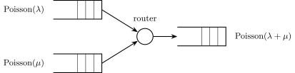
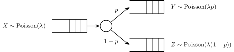
23264 words